
Cost Management: A Strategic Emphasis 5th Edition by David Stout, Edward Blocher, Gary Cokins
Edition 5ISBN: 0073526940Cost Management: A Strategic Emphasis 5th Edition by David Stout, Edward Blocher, Gary Cokins
Edition 5ISBN: 0073526940Regression Analysis: Cross-Sectional Analysis; Calculation of a Regression Equation Jim Manzano is the general partner of an investment group that owns a number of commercial and industrial properties, including a chain of 15 convenience stores located in the greater metropolitan area of Cleveland, Ohio. Jim is concerned about the recent increase in inventory theft and waste (he calls it “spoilage”) in his stores. Spoilage has increased by more than 20 percent in each of the past two years. In some stores, the main reason is theft; in others, it is damage and vandalism; and in still others, merchandise actually does spoil and must be thrown out. Jim has collected data on spoilage at each of his stores in the recent month and is looking for patterns of spoilage relative to store size (measured by square feet of floor space, number of employees, and total sales) and to the location of the store (location 1 is an area where few arrests for theft, disorderly conduct, or vandalism are made, and location 3 is for areas with high arrests). Jim is not sure, but he suspects, based on his experience managing convenience stores, that a relationship exists among these factors. A colleague told him that a type of regression called “cross-sectional” regression would suit his needs. The cross-sectional regression takes data from a single time period and determines predictions for the dependent variable at different cost objects (in this case, different stores). The objective of the cross-sectional regression is to compare the actual known value for the dependent variable to the predicted value as a basis for assessing the reasonableness of the actual value. This approach is often used in cases similar to Jim’s in which the accuracy or reasonableness of the reported dependent variable is a concern. In effect, the cross-sectional regression develops a model that represents the overall patterns in all the data, and the unusual stores will be identified by the largest error terms in the regression. The following data are for the most recent month’s operations:
Store Number | Inventory Spoilage | Square Footage | Number of Employees | Location | Sales |
1 | $1,512 | 2,400 | 8 | 1 | $312,389 |
2 | 3,005 | 3,900 | 10 | 2 | 346,235 |
3 | 1,686 | 3,200 | 12 | 1 | 376,465 |
4 | 1,908 | 3,400 | 12 | 1 | 345,723 |
5 | 2,384 | 3,750 | 9 | 2 | 453,983 |
6 | 4,806 | 4,800 | 10 | 3 | 502,984 |
7 | 2,253 | 3,500 | 8 | 1 | 325,436 |
8 | 1 ,443 | 3,000 | 10 | 1 | 253,647 |
9 | 3,755 | 5,550 | 15 | 2 | 562,534 |
10 | 1,023 | 2,250 | 15 | 1 | 287,364 |
11 | 1,552 | 2,500 | 9 | 1 | 198,374 |
12 | 2,119 | 3,500 | 16 | 2 | 333,984 |
13 | 5,506 | 7,500 | 15 | 3 | 673,345 |
14 | 3,034 | 5,700 | 16 | 2 | 588,947 |
15 | 772 | 2,200 | 8 | 1 | 225,364 |
Totals | $36,758 | 57,150 | 173 |
| $5,786,774 |
Required
1. Using Excel or an equivalent software program, prepare a regression analysis that predicts inventory spoilage at each of the 15 stores. Use any of the four potential independent variables (or a combination) you think appropriate and explain your answer. Also evaluate the precision and reliability of the regression you select.
2. Using the regression equation you developed in requirement 1, determine which of the 15 stores might have inventory spoilage that is out of line relative to the entire chain of stores. Explain your choice.
Step 1 of 2
Cross-sectional Regression (60 min)
1.?The first regression we try includes all four independent variables; square feet, number of employees, location type, and sales dollars. Each of these variables has a plausible relationship to inventory spoilage. We find from the regression results (see below) that the R-squared is very good (95%), the SE is relatively poor at 15% = 370.51/(36,758/15). The t-values are good for two of the variables (location and square feet), poor for the sales variable, and marginal for the number of employees variable.
Variable | t-value |
Square Feet | 2.86 |
Employees | -1.89 |
Location | 3.63 |
Sales | -.33 |
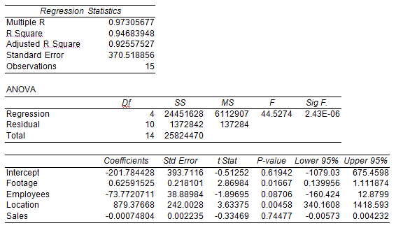
The negative t-value on “employees” suggests that the spoilage at some stores might be due to under-staffing, but the t-value is not strong enough for strong conclusions. The t-value on “sales” is weak enough that we should consider deleting the variable from the model; moreover, can we explain why the coefficient on this variable is negative? With this thinking, we decide to re-run the model keeping only the two independent variables: location and square feet. The results are shown below, under “Regression Two.”
The second regression, shown below, has comparable values for R-squared and SE, but the t-values are improved. Additionally, the F-value almost doubles, meaning a more statistically reliable model. For these reasons we have chosen to rely on this second regression model to complete the analysis for Jim. Note below the regression results there is a residual report which shows the predicted and actual values for spoilage at each store, and the error term (“residual”). A large positive residual is unfavorable while a large negative residual is favorable.
Step 2 of 2
Why don’t you like this exercise?
Other


