
Introductory Econometrics: A Modern Approach 6th Edition by Jeffrey M Wooldridge
Edition 6ISBN: 130527010XIntroductory Econometrics: A Modern Approach 6th Edition by Jeffrey M Wooldridge
Edition 6ISBN: 130527010XThis question assumes that you have access to a statistical package the computes standard errors robust to arbitrary serial correlation and heteroskedasticity for panel data methods.
(i) For the pooled OLS estimates in Table, obtain the standard errors that allow for arbitrary serial correlation (in the composite errors, vit = ai + uit) and het-eroskedasticity. How do the robust standard errors for educ, married, and union compare with the nonrobust ones?
(ii) Now obtain the robust standard errors for the fixed effects estimates that allow arbitrary serial correlation and heteroskedasticity in the idiosyncratic errors, uit. How do these compare with the nonrobust FE standard errors?
(iii) For which method, pooled OLS or FE, is adjusting the standard errors for serial correlation more important? Why?
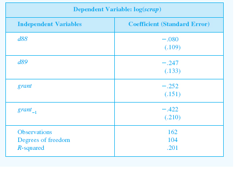
Table Fixed Effects Estimation of Scrap Rate Equation
Step 1 of 5
(i)
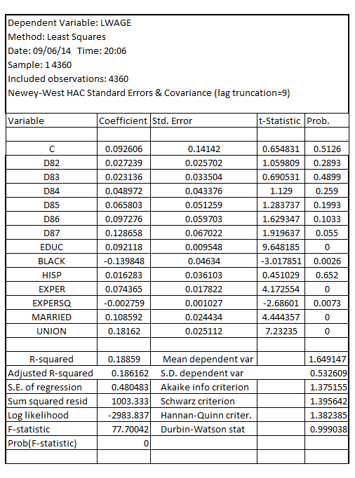
Estimating the wage equation in which is the dependent variable and
 , the year dummy variables as the explanatory variables along with
  as the other explanatory variables, assuming the standard error for the coefficients of the explanatory variables that allow for the arbitrary serial correlation and heteroscedasticity and assuming
  as the base dummy year, the result is:
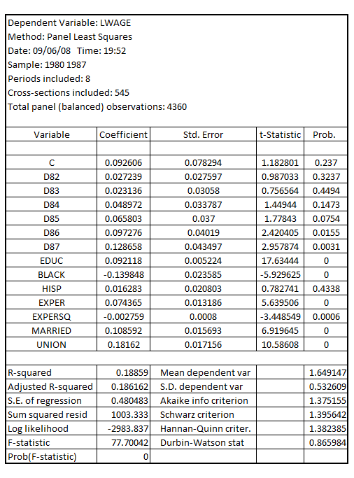
Estimating the wage equation in which is the dependent variable and
 , the year dummy variables as the explanatory variables along with
  as the other explanatory variables, assuming usual OLS standard error and assuming
  as the base dummy year, the result is:
On comparing the robust standard errors for  with the non-robust errors, the result is:
Step 2 of 5
Step 3 of 5
Step 4 of 5
Step 5 of 5
Why don’t you like this exercise?
Other


