Introductory Econometrics: A Modern Approach 6th Edition by Jeffrey M Wooldridge

Exercise 15

VOTE2.RAW includes panel data on House of Representative elections in 1988 and 1990. Only winners from 1988 who are also running in 1990 appear in the sample; these are the incumbents. An unobserved effects model explaining the share of the incumbent's vote in terms of expenditures by both candidates is

vote.t = ?0+ ?0d90t +?log(inexpit) + ?log(chexpiit) + ?3incshrit + ai + uit,

where incshrtt is the incumbent's share of total campaign spending (in percentage form). The unobserved effect a. contains characteristics of the incumbent—such as "quality"—as well as things about the district that are constant. The incumbent's gender and party are constant over time, so these are subsumed in ai. We are interested in the effect of campaign expenditures on election outcomes.

(i) Difference the given equation across the two years and estimate the differenced equation by OLS. Which variables are individually significant at the 5% level against a two-sided alternative?

(ii) In the equation from part (i), test for joint significance of Alog(inexp) and Alog(chexp). Report the p-value.

(iii) Reestimate the equation from part (i) using Aincshr as the only independent variable. Interpret the coefficient on Aincshr. For example, if the incumbent's share of spending increases by 10 percentage points, how is this predicted to affect the incumbent's share of the vote?

(iv) Redo part (iii), but now use only the pairs that have repeat challengers. [This allows us to control for characteristics of the challengers as well, which would be in ai. Levitt (1994) conducts a much more extensive analysis.]

Step 1 of 5

(i)

For the year 1988, the unobserved effects model is given by:

For the year 1990, the unobserved effects model is given by:

On differencing the given equations across the two years, the model is:

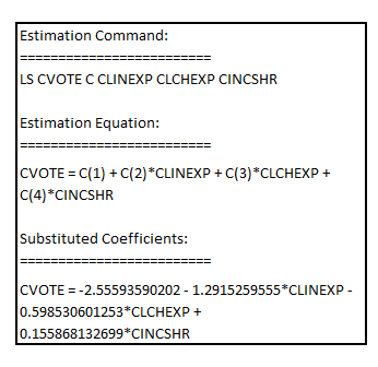
On estimating this model by OLS, the result is:

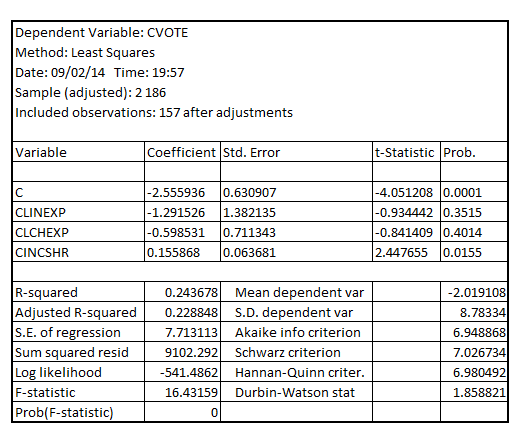
The coefficient of the explanatory variable has the p-value 0.0155 which is less than the critical p-value of 0.05 at 5% level of significance, thereby, indicating that this variable is individually significant at the 5% level of significance.

Rest of the explanatory variables is not statistically significant as their respective p-value is greater than the critical p-value of 0.05 at 5% level of significance.