
Introductory Econometrics: A Modern Approach 6th Edition by Jeffrey M Wooldridge
Edition 6ISBN: 130527010XIntroductory Econometrics: A Modern Approach 6th Edition by Jeffrey M Wooldridge
Edition 6ISBN: 130527010X(i) In Computer Exercise, you estimated a simple relationship between consumption growth and growth in disposable income. Test the equation for AR(1) serial correlation (using CONSUMP.RAW).
(ii) In Computer Exercise, you tested the permanent income hypothesis by regressing the growth in consumption on one lag. After running this regression, test for heteroskedasticity by regressing the squared residuals on gct-1 and gct-12 . What do you conclude?
Exercise Use the data set CONSUMP.RAW for this exercise.
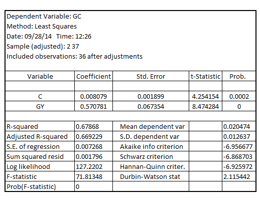
(i) Estimate a simple regression model relating the growth in real per capita consumption (of nondurables and services) to the growth in real per capita disposable income. Use the change in the logarithms in both cases. Report the results in the usual form. Interpret the equation and discuss statistical significance.
(ii) Add a lag of the growth in real per capita disposable income to the equation from part (i). What do you conclude about adjustment lags in consumption growth?
(iii) Add the real interest rate to the equation in part (i). Does it affect consumption growth?
Exercise Use CONSUMP.RAW for this exercise. One version of the permanent income hypothesis (PIH) of consumption is that the growth in consumption is unpredictable. [Another version is that the change in consumption itself is unpredictable; see Mankiw (1994, Chapter 15) for discussion of the PIH.] Let gct = log(ct) -log(ct-1) be the growth in real per capita consumption (of nondurables and services). Then the PIH implies that E![<blockquote> (i) In Computer Exercise, you estimated a simple relationship between consumption growth and growth in disposable income. Test the equation for AR(1) serial correlation (using CONSUMP.RAW). (ii) In Computer Exercise, you tested the permanent income hypothesis by regressing the growth in consumption on one lag. After running this regression, test for heteroskedasticity by regressing the squared residuals on gc<span class=sub>t-1</span> and gc<span class=sub>t-1</span><span class=sup>2</span> . What do you conclude? </blockquote> Exercise Use the data set CONSUMP.RAW for this exercise. <blockquote> (i) Estimate a simple regression model relating the growth in real per capita consumption (of nondurables and services) to the growth in real per capita disposable income. Use the change in the logarithms in both cases. Report the results in the usual form. Interpret the equation and discuss statistical significance. (ii) Add a lag of the growth in real per capita disposable income to the equation from part (i). What do you conclude about adjustment lags in consumption growth? (iii) Add the real interest rate to the equation in part (i). Does it affect consumption growth? </blockquote> Exercise Use CONSUMP.RAW for this exercise. One version of the permanent income hypothesis (PIH) of consumption is that the growth in consumption is unpredictable. [Another version is that the change in consumption itself is unpredictable; see Mankiw (1994, Chapter 15) for discussion of the PIH.] Let gc<span class=sub>t</span> = log(c<span class=sub>t</span>) -log(c<span class=sub>t-1</span>) be the growth in real per capita consumption (of nondurables and services). Then the PIH implies that E = E(gc<span class=sub>t</span>), where I<span class=sub>t-1</span> denotes information known at time (t-1); in this case, t denotes a year. <blockquote> (i) Test the PIH by estimating gc<span class=sub>t</span> = ?<span class=sub>0</span> + ?<span class=sub>1</span>gc<span class=sub>t-1</span> + u<span class=sub>t</span>. Clearly state the null and alternative hypotheses. What do you conclude? (ii) To the regression in part (i), add gy<span class=sub>t-1</span> and i3<span class=sub>t-1</span>, where gyt is the growth in real per capita disposable income and i3t is the interest rate on three-month T-bills; note that each must be lagged in the regression. Are these two additional variables jointly significant? </blockquote>](https://d2lvgg3v3hfg70.cloudfront.net/SMCC2709/a5e050b4_d7e2_46c8_96a9_2c8f682c0dc9_SMCC2709_11.jpg) = E(gct), where It-1 denotes information known at time (t-1); in this case, t denotes a year.
= E(gct), where It-1 denotes information known at time (t-1); in this case, t denotes a year.
(i) Test the PIH by estimating gct = ?0 + ?1gct-1 + ut. Clearly state the null and alternative hypotheses. What do you conclude?
(ii) To the regression in part (i), add gyt-1 and i3t-1, where gyt is the growth in real per capita disposable income and i3t is the interest rate on three-month T-bills;
note that each must be lagged in the regression. Are these two additional variables jointly significant?
Step 1 of 3
(i)
Estimate the simple relationship between consumption growth and growth of the real per capita disposable income, the result is:

Now estimate the error term and regress it on
 , the result is:

It shall be observed that the coefficient of  is with the p-value 0.6201 which is greater than the critical p-value of 0.05 at 5% level of significance indicating that there is no statistically significant AR (1) serial correlation in the error term
Step 2 of 3
Step 3 of 3
Why don’t you like this exercise?
Other


