
Introductory Econometrics: A Modern Approach 6th Edition by Jeffrey M Wooldridge
Edition 6ISBN: 130527010XIntroductory Econometrics: A Modern Approach 6th Edition by Jeffrey M Wooldridge
Edition 6ISBN: 130527010XUse the data set in BEAUTY.RAW, which contains a subset of the variables (but more usable observations than in the regressions) reported by Hamermesh and Biddle (1994).
(i) Find the separate fractions of men and women that are classified as having above average looks. Are more people rated as having above average or below average looks?
(ii) Test the null hypothesis that the population fractions of above-average-looking women and men are the same. Report the one-sided p-value that the fraction is higher for women. (Hint: Estimating a simple linear probability model is easiest.)
(iii) Now estimate the model

separately for men and women, and report the results in the usual form. In both cases, interpret the coefficient on belavg. Explain in words what the hypothesis H0:  against H1:
  means, and find the p-values for men and women.
(iv) Is there convincing evidence that women with above average looks earn more than women with average looks? Explain.
(v) For both men and women, add the explanatory variables educ, exper, exper2, union, goodhlth, black, married, south, bigcity, smllcity, and service. Do the effects of the “looks” variables change in important ways?
(vi) Use the SSR form of the Chow F statistic to test whether the slopes of the regression functions in part (v) differ across men and women. Be sure to allow for an intercept shift under the null.
Step 1 of 27
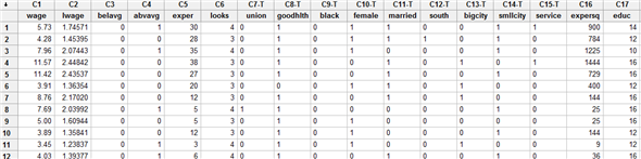
Consider the provided data set “BEAUTY” to solve the subparts and write down the whole data in to Minitab worksheet, the screenshot is shown below:
Step 2 of 27
Step 3 of 27
Step 4 of 27
Step 5 of 27
Step 6 of 27
Step 7 of 27
Step 8 of 27
Step 9 of 27
Step 10 of 27
Step 11 of 27
Step 12 of 27
Step 13 of 27
Step 14 of 27
Step 15 of 27
Step 16 of 27
Step 17 of 27
Step 18 of 27
Step 19 of 27
Step 20 of 27
Step 21 of 27
Step 22 of 27
Step 23 of 27
Step 24 of 27
Step 25 of 27
Step 26 of 27
Step 27 of 27
Why don’t you like this exercise?
Other


