Deck 10: Mathematical Modeling and Variation
Full screen (f)
Question
Question
An overhead garage door has two springs,one on each side of the door (see figure).A force of pounds is required to stretch each spring 1 foot.Because of a pulley system,the springs stretch only one-half the distance the door travels.The door moves a total of feet,and the springs are at their natural length when the door is open.Find the combined lifting force applied to the door by the springs when the door is closed. 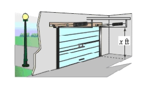
A)
B)
C)
D)
E)
A)
B)
C)
D)
E)
Question
Question
Question
Question
Question
Question
Question
Question
Question
Question
Question
Question
Question
Question
Question
Question
Question
A force of newtons stretches a spring meter (see figure). 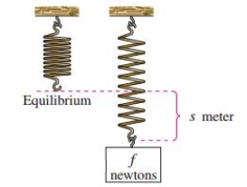 How far will a force of 60 newtons stretch the spring? What force is required to stretch the spring 0.1 meter?
A)
B)
C)
D)
E)
How far will a force of 60 newtons stretch the spring? What force is required to stretch the spring 0.1 meter? A)
B)
C)
D)
E)
Question
Question
Question
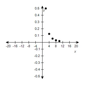
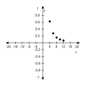
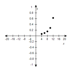
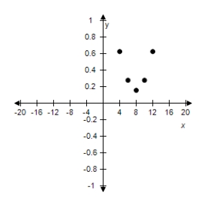
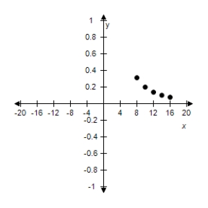
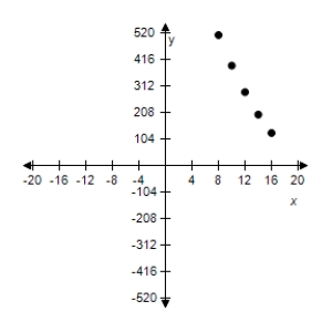
Use the given value of k to complete the table for the inverse variation model Plot the points on a rectangular coordinate system.
A)
B)

C)
D)
E)
A)
B)
C)
D)
E)
Question
Question
Question
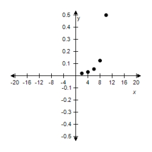
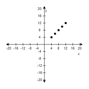
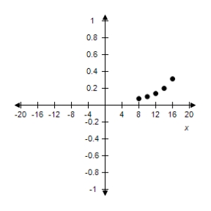
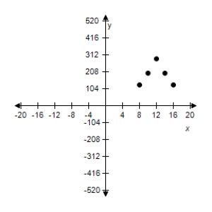
Use the given value of k to complete the table for the direct variation model .
Plot the points on a rectangular coordinate system.
A)
B)

C)

D)
E)
Plot the points on a rectangular coordinate system.
A)
B)
C)
D)
E)
Question
Question
Question
Question
Question
Question
Use the given value of k to complete the table for the inverse variation model Plot the points on a rectangular coordinate system.
A)

B)
C)
D)
E)
A)
B)
C)
D)
E)
Question
Use the given value of k to complete the table for the direct variation model .
Plot the points on a rectangular coordinate system.
A)
B)
C)
D)

E)

Plot the points on a rectangular coordinate system.
A)
B)
C)
D)
E)
Question
Use the given value of k to complete the table for the inverse variation model Plot the points on a rectangular coordinate system.
A)
B)

C)
D)
E)
A)
B)
C)
D)
E)
Question
Question
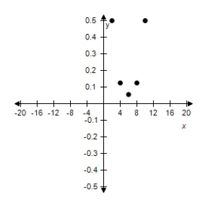
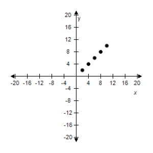
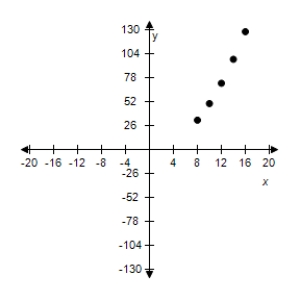
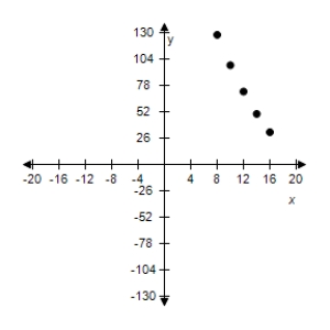
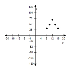
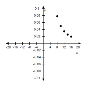
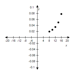
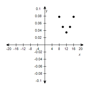
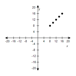
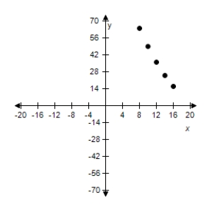
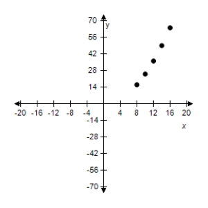
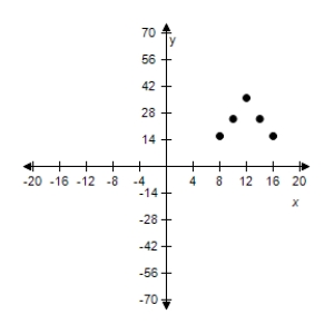
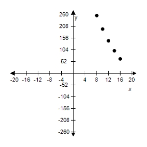
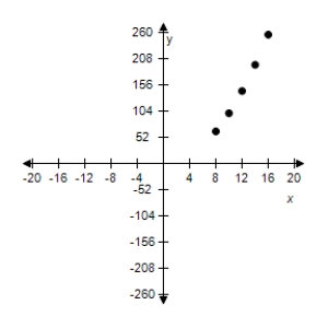
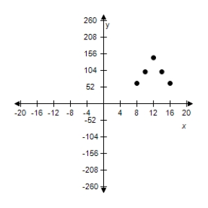
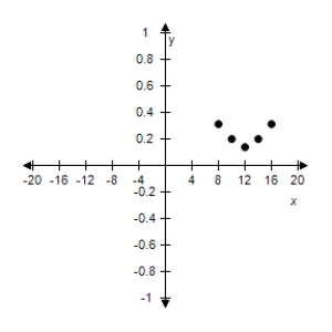
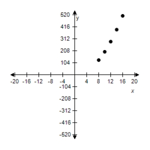
An oceanographer took readings of the water temperatures C (in degrees Celsius)at several depths d (in meters).The data collected are shown in the table.
Sketch a scatter plot of the data.
A)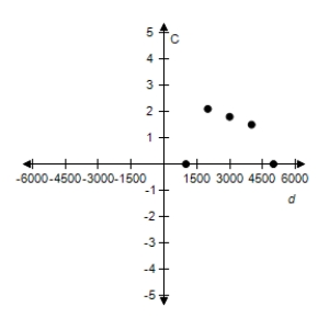
B)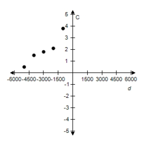
C)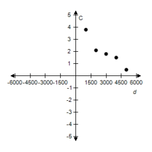
D)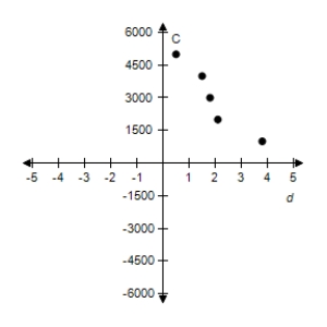
E)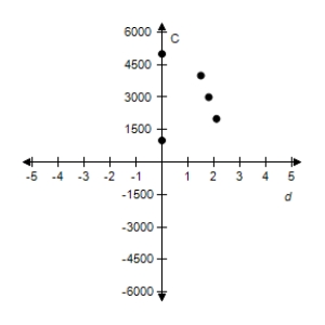
Sketch a scatter plot of the data.
A)
B)
C)
D)
E)
Question
Question
Use the given value of k to complete the table for the direct variation model .
Plot the points on a rectangular coordinate system.
A)
B)
C)

D)
E)

Plot the points on a rectangular coordinate system.
A)
B)
C)
D)
E)
Question
Use the given value of k to complete the table for the inverse variation model . Plot the points on a rectangular coordinate system.
A)
B)

C)
D)
E)

A)
B)
C)
D)
E)
Question
Question
Use the given value of k to complete the table for the direct variation model .
Plot the points on a rectangular coordinate system.
A)
B)

C)

D)
E)
Plot the points on a rectangular coordinate system.
A)
B)
C)
D)
E)
Question
Question
Question
Question
Question
Question
Question
Question
Question

Unlock Deck
Sign up to unlock the cards in this deck!
Unlock Deck
Unlock Deck
1/49
Play
Full screen (f)
Deck 10: Mathematical Modeling and Variation
1
The simple interest on an investment is directly proportional to the amount of the investment.By investing $2400 in a certain bond issue,you obtained an interest payment of $111.75 after 1 year.Find a mathematical model that gives the interest I for this bond issue after 1 year in terms of the amount invested P.(Round your answer to three decimal places. )
A)
B)
C)
D)
E)
A)
B)
C)
D)
E)
2
An overhead garage door has two springs,one on each side of the door (see figure).A force of pounds is required to stretch each spring 1 foot.Because of a pulley system,the springs stretch only one-half the distance the door travels.The door moves a total of feet,and the springs are at their natural length when the door is open.Find the combined lifting force applied to the door by the springs when the door is closed.
A)
B)
C)
D)
E)
A)
B)
C)
D)
E)
3
The simple interest on an investment is directly proportional to the amount of the investment.By investing $5800 in a municipal bond,you obtained an interest payment of $221.25 after 1 year.Find a mathematical model that gives the interest I for this municipal bond after 1 year in terms of the amount invested P.(Round your answer to three decimal places. )
A)
B)
C)
D)
E)
A)
B)
C)
D)
E)
4
Find a mathematical model representing the statement.(Determine the constant of proportionality. )
Y varies inversely as x.
A)
B)
C)
D)
E)
Y varies inversely as x.
A)
B)
C)
D)
E)
Unlock Deck
Unlock for access to all 49 flashcards in this deck.
Unlock Deck
k this deck
5
On a yardstick with scales in inches and centimeters,you notice that 11 inches is approximately the same length as 33 centimeters.Use this information to find a mathematical model that relates centimeters y to inches x.Then use the model to find the numbers of centimeters in 60 inches and 70 inches.(Round your answer to one decimal place. )
A)Model: y = x;20 cm,23.3 cm
B)Model: y = 3x;180 cm,23.3 cm
C)Model: y = 3x;20 cm,210 cm
D)Model: y = 3x;180 cm,210 cm
E)Model: y = x;180 cm,210 cm
A)Model: y = x;20 cm,23.3 cm
B)Model: y = 3x;180 cm,23.3 cm
C)Model: y = 3x;20 cm,210 cm
D)Model: y = 3x;180 cm,210 cm
E)Model: y = x;180 cm,210 cm
Unlock Deck
Unlock for access to all 49 flashcards in this deck.
Unlock Deck
k this deck
6
Find a mathematical model representing the statement.(Determine the constant of proportionality. )
P varies directly as x and inversely as the square of y.(P = when x = 25 and y = 10. )
A)
B)
C)
D)
E)
P varies directly as x and inversely as the square of y.(P = when x = 25 and y = 10. )
A)
B)
C)
D)
E)
Unlock Deck
Unlock for access to all 49 flashcards in this deck.
Unlock Deck
k this deck
7
Property tax is based on the assessed value of a property.A house that has an assessed value of $200,000 has a property tax of $4,820.Find a mathematical model that gives the amount of property tax y in terms of the assessed value x of the property.Use the model to find the property tax on a house that has an assessed value of $230,000.(Round your answer to four decimal places. )
A)
B)
C)
D)
E)
A)
B)
C)
D)
E)
Unlock Deck
Unlock for access to all 49 flashcards in this deck.
Unlock Deck
k this deck
8
Find a mathematical model representing the statement.(Determine the constant of proportionality. )
F is jointly proportional to r and the third power of s.
A)
B)
C)
D)
E)
F is jointly proportional to r and the third power of s.
A)
B)
C)
D)
E)
Unlock Deck
Unlock for access to all 49 flashcards in this deck.
Unlock Deck
k this deck
9
Assume that y is directly proportional to x.Use the given x-value and y-value to find a linear model that relates y and x.
A)
B)
C)
D)
E)
A)
B)
C)
D)
E)
Unlock Deck
Unlock for access to all 49 flashcards in this deck.
Unlock Deck
k this deck
10
Find a mathematical model representing the statement.(Determine the constant of proportionality. )
Y is inversely proportional to x.
A)
B)
C)
D)
E)
Y is inversely proportional to x.
A)
B)
C)
D)
E)
Unlock Deck
Unlock for access to all 49 flashcards in this deck.
Unlock Deck
k this deck
11
The work W (in joules)done when lifting an object varies jointly with the mass m (in kilograms)of the object and the height h (in meters)that the object is lifted.The work done when a 120-kilogram object is lifted 1.8 meters is 2116.8 joules.How much work is done when lifting a 200-kilogram object 1.5 meters?
A)2960 J
B)2920 J
C)2940 J
D)2950 J
E)2930 J
A)2960 J
B)2920 J
C)2940 J
D)2950 J
E)2930 J
Unlock Deck
Unlock for access to all 49 flashcards in this deck.
Unlock Deck
k this deck
12
Assume that y is directly proportional to x.Use the given x-value and y-value to find a linear model that relates y and x.
A)y = 76x
B)y = - 76x
C)y = x
D)y = - x
E)y = - 380x
A)y = 76x
B)y = - 76x
C)y = x
D)y = - x
E)y = - 380x
Unlock Deck
Unlock for access to all 49 flashcards in this deck.
Unlock Deck
k this deck
13
The coiled spring of a toy supports the weight of a child.The spring is compressed a distance of 1.6 inches by the weight of a 35-pound child.The toy will not work properly if its spring is compressed more than 6 inches.What is the weight of the heaviest child who should be allowed to use the toy? (Round your answer to two decimal places. )
A)136.25 lb
B)126.25 lb
C)131.25 lb
D)35 lb
E)141.25 lb
A)136.25 lb
B)126.25 lb
C)131.25 lb
D)35 lb
E)141.25 lb
Unlock Deck
Unlock for access to all 49 flashcards in this deck.
Unlock Deck
k this deck
14
A force of 270 newtons stretches a spring 0.18 meter.What force is required to stretch the spring 0.19 meter?
A)295 N
B)290 N
C)285 N
D)280 N
E)270 N
A)295 N
B)290 N
C)285 N
D)280 N
E)270 N
Unlock Deck
Unlock for access to all 49 flashcards in this deck.
Unlock Deck
k this deck
15
Assume that y is directly proportional to x.Use the given x-value and y-value to find a linear model that relates y and x.
A)y = x
B)y = - 2400x
C)y = x
D)y = - x
E)y = - x
A)y = x
B)y = - 2400x
C)y = x
D)y = - x
E)y = - x
Unlock Deck
Unlock for access to all 49 flashcards in this deck.
Unlock Deck
k this deck
16
Find a mathematical model representing the statement.(Determine the constant of proportionality. )
Z varies jointly as x and y.
A)
B)
C)
D)
E)
Z varies jointly as x and y.
A)
B)
C)
D)
E)
Unlock Deck
Unlock for access to all 49 flashcards in this deck.
Unlock Deck
k this deck
17
When buying gasoline,you notice that 16 gallons of gasoline is approximately the same amount of gasoline as 51 liters.Use this information to find a linear model that relates liters y to gallons x.Then use the model to find the numbers of liters in 25 gallons and 45 gallons. (Round your answer to one decimal place. )
A)Model: y = x;7.8 L,14.1 L
B)Model: y = x;79.7 L,14.1 L
C)Model: y = x;7.8 L,143.4 L
D)Model: y = x;79.7 L,143.4 L
E)Model: y = x;79.7 L,143.4 L
A)Model: y = x;7.8 L,14.1 L
B)Model: y = x;79.7 L,14.1 L
C)Model: y = x;7.8 L,143.4 L
D)Model: y = x;79.7 L,143.4 L
E)Model: y = x;79.7 L,143.4 L
Unlock Deck
Unlock for access to all 49 flashcards in this deck.
Unlock Deck
k this deck
18
State sales tax is based on retail price.An item that sells for $180.99 has a sales tax of $17.4.Find a mathematical model that gives the amount of sales tax y in terms of the retail price x.Use the model to find the sales tax on a $589.99 purchase.(Round your answer to four decimal places. )
A)
B)
C)
D)
E)
A)
B)
C)
D)
E)
Unlock Deck
Unlock for access to all 49 flashcards in this deck.
Unlock Deck
k this deck
19
A force of newtons stretches a spring meter (see figure). How far will a force of 60 newtons stretch the spring? What force is required to stretch the spring 0.1 meter?
A)
B)
C)
D)
E)
How far will a force of 60 newtons stretch the spring? What force is required to stretch the spring 0.1 meter? A)
B)
C)
D)
E)
Unlock Deck
Unlock for access to all 49 flashcards in this deck.
Unlock Deck
k this deck
20
Assume that y is directly proportional to x.Use the given x-value and y-value to find a linear model that relates y and x.
A)
B)
C)
D)
E)
A)
B)
C)
D)
E)
Unlock Deck
Unlock for access to all 49 flashcards in this deck.
Unlock Deck
k this deck
21
Find a mathematical model representing the statement.(Determine the constant of proportionality. )
V varies jointly as p and q and inversely as the square of s.(ν = 1.4 when p = 4.4,q = 7.3 and s = 1.8. )
A)
B)
C)
D)
E)
V varies jointly as p and q and inversely as the square of s.(ν = 1.4 when p = 4.4,q = 7.3 and s = 1.8. )
A)
B)
C)
D)
E)
Unlock Deck
Unlock for access to all 49 flashcards in this deck.
Unlock Deck
k this deck
22
Use the given value of k to complete the table for the inverse variation model Plot the points on a rectangular coordinate system.
A)
B)
C)
D)
E)
A)
B)
C)
D)
E)
Unlock Deck
Unlock for access to all 49 flashcards in this deck.
Unlock Deck
k this deck
23
Determine whether the variation model below is of the form or . x
13
26
39
52
65
Y
3
6
9
12
15
A)
B)
13
26
39
52
65
Y
3
6
9
12
15
A)
B)
Unlock Deck
Unlock for access to all 49 flashcards in this deck.
Unlock Deck
k this deck
24
Use the fact that the resistance of a wire carrying an electrical current is directly proportional to its length and inversely proportional to its cross-sectional area.
A 10-foot piece of copper wire produces a resistance of 0.2 ohm.Use the constant of proportionality k = 0.000833 to find the diameter of the wire.
(Round the answer up to three decimal places. )
A)0.23 ft
B)0.58 ft
C)0.38 ft
D)0.48 ft
E)0.73 ft
A 10-foot piece of copper wire produces a resistance of 0.2 ohm.Use the constant of proportionality k = 0.000833 to find the diameter of the wire.
(Round the answer up to three decimal places. )
A)0.23 ft
B)0.58 ft
C)0.38 ft
D)0.48 ft
E)0.73 ft
Unlock Deck
Unlock for access to all 49 flashcards in this deck.
Unlock Deck
k this deck
25
Use the given value of k to complete the table for the direct variation model .
Plot the points on a rectangular coordinate system.
A)
B)
C)
D)
E)
Plot the points on a rectangular coordinate system.
A)
B)
C)
D)
E)
Unlock Deck
Unlock for access to all 49 flashcards in this deck.
Unlock Deck
k this deck
26
Find a mathematical model representing the statement.(Determine the constant of proportionality. )
Z varies directly as the square of x and inversely as y.(z = 36 when x = 9 and y = 3. )
A)
B)
C)
D)
E)
Z varies directly as the square of x and inversely as y.(z = 36 when x = 9 and y = 3. )
A)
B)
C)
D)
E)
Unlock Deck
Unlock for access to all 49 flashcards in this deck.
Unlock Deck
k this deck
27
Determine whether the variation model is of the form or and find k.Then write a model that relates y and x.
A)
B)
C)
D)
E)
A)
B)
C)
D)
E)
Unlock Deck
Unlock for access to all 49 flashcards in this deck.
Unlock Deck
k this deck
28
The frequency of vibrations of a piano string varies directly as the square root of the tension on the string and inversely as the length of the string.The middle A string has a frequency of 430 vibrations per second.Find the frequency of a string that has 1.25 times as much tension and is 1.4 times as long.
A)373.4 vibrations / sec
B)343.4 vibrations / sec
C)353.4 vibrations / sec
D)383.4 vibrations / sec
E)363.4 vibrations / sec
A)373.4 vibrations / sec
B)343.4 vibrations / sec
C)353.4 vibrations / sec
D)383.4 vibrations / sec
E)363.4 vibrations / sec
Unlock Deck
Unlock for access to all 49 flashcards in this deck.
Unlock Deck
k this deck
29
Use the fact that the diameter of the largest particle that can be moved by a stream varies approximately directly as the square of the velocity of the stream.
A stream with a velocity of mile per hour can move coarse sand particles about 0.07 inch in diameter.Approximate the velocity required to carry particles 0.2 inch in diameter.(Round your answer to two decimal places. )
A)About 0.84 mi/h
B)About 0.19 mi/h
C)About -0.16 mi/h
D)About 0.49 mi/h
E)About 0.34 mi/h
Unlock Deck
Unlock for access to all 49 flashcards in this deck.
Unlock Deck
k this deck
30
Use the fact that the resistance of a wire carrying an electrical current is directly proportional to its length and inversely proportional to its cross-sectional area.
If #28 copper wire (which has a diameter of 0.0126 inch)has a resistance of 68.17 ohms per thousand feet,what length of #28 copper wire will produce a resistance of 30.5 ohms?
A)About 447 ft
B)About 442 ft
C)About 432 ft
D)About 452 ft
E)About 462 ft
If #28 copper wire (which has a diameter of 0.0126 inch)has a resistance of 68.17 ohms per thousand feet,what length of #28 copper wire will produce a resistance of 30.5 ohms?
A)About 447 ft
B)About 442 ft
C)About 432 ft
D)About 452 ft
E)About 462 ft
Unlock Deck
Unlock for access to all 49 flashcards in this deck.
Unlock Deck
k this deck
31
Use the given value of k to complete the table for the inverse variation model Plot the points on a rectangular coordinate system.
A)
B)
C)
D)
E)
A)
B)
C)
D)
E)
Unlock Deck
Unlock for access to all 49 flashcards in this deck.
Unlock Deck
k this deck
32
Use the given value of k to complete the table for the direct variation model .
Plot the points on a rectangular coordinate system.
A)
B)
C)
D)
E)
Plot the points on a rectangular coordinate system.
A)
B)
C)
D)
E)
Unlock Deck
Unlock for access to all 49 flashcards in this deck.
Unlock Deck
k this deck
33
Use the given value of k to complete the table for the inverse variation model Plot the points on a rectangular coordinate system.
A)
B)
C)
D)
E)
A)
B)
C)
D)
E)
Unlock Deck
Unlock for access to all 49 flashcards in this deck.
Unlock Deck
k this deck
34
Determine whether the variation model is of the form or and find k.Then write a model that relates y and x.
A)
B)
C)
D)
E)
A)
B)
C)
D)
E)
Unlock Deck
Unlock for access to all 49 flashcards in this deck.
Unlock Deck
k this deck
35
An oceanographer took readings of the water temperatures C (in degrees Celsius)at several depths d (in meters).The data collected are shown in the table.
Sketch a scatter plot of the data.
A)
B)
C)
D)
E)
Sketch a scatter plot of the data.
A)
B)
C)
D)
E)
Unlock Deck
Unlock for access to all 49 flashcards in this deck.
Unlock Deck
k this deck
36
Determine whether the variation model is of the form or and find k.Then write a model that relates y and x.
A)
B)
C)
D)
E)
A)
B)
C)
D)
E)
Unlock Deck
Unlock for access to all 49 flashcards in this deck.
Unlock Deck
k this deck
37
Use the given value of k to complete the table for the direct variation model .
Plot the points on a rectangular coordinate system.
A)
B)
C)
D)
E)
Plot the points on a rectangular coordinate system.
A)
B)
C)
D)
E)
Unlock Deck
Unlock for access to all 49 flashcards in this deck.
Unlock Deck
k this deck
38
Use the given value of k to complete the table for the inverse variation model . Plot the points on a rectangular coordinate system.
A)
B)
C)
D)
E)
A)
B)
C)
D)
E)
Unlock Deck
Unlock for access to all 49 flashcards in this deck.
Unlock Deck
k this deck
39
Determine whether the variation model is of the form or and find k.Then write a model that relates y and x.
A)
B)
C)
D)
E)
A)
B)
C)
D)
E)
Unlock Deck
Unlock for access to all 49 flashcards in this deck.
Unlock Deck
k this deck
40
Use the given value of k to complete the table for the direct variation model .
Plot the points on a rectangular coordinate system.
A)
B)
C)
D)
E)
Plot the points on a rectangular coordinate system.
A)
B)
C)
D)
E)
Unlock Deck
Unlock for access to all 49 flashcards in this deck.
Unlock Deck
k this deck
41
After determining whether the variation model below is of the form or ,find the value of k.
A)
B)
C)
D)
E)
A)
B)
C)
D)
E)
Unlock Deck
Unlock for access to all 49 flashcards in this deck.
Unlock Deck
k this deck
42
The simple interest on an investment is directly proportional to the amount of the investment.By investing $6000 in a certain certificate of deposit,you obtained an interest payment of $276.00 after 1 year.Determine a mathematical model that gives the interest,I ,for this CD after 1 year in terms of the amount invested,P.
A)
B)
C)
D)
E)
A)
B)
C)
D)
E)
Unlock Deck
Unlock for access to all 49 flashcards in this deck.
Unlock Deck
k this deck
43
Find a mathematical model for the verbal statement: "m varies directly as the square of w and inversely as s."
A)
B)
C)
D)
E)
A)
B)
C)
D)
E)
Unlock Deck
Unlock for access to all 49 flashcards in this deck.
Unlock Deck
k this deck
44
Find a mathematical model for the verbal statement:
"Q is jointly proportional to the cube of h and the square root of m."
A)
B)
C)
D)
E)
"Q is jointly proportional to the cube of h and the square root of m."
A)
B)
C)
D)
E)
Unlock Deck
Unlock for access to all 49 flashcards in this deck.
Unlock Deck
k this deck
45
Hooke's law states that the magnitude of force,F,required to stretch a spring x units beyond its natural length is directly proportional to x.If a force of 3 pounds stretches a spring from its natural length of 10 inches to a length of 10.7 inches,what force will stretch the spring to a length of 11.5 inches? Round your answer to the nearest hundredth.
A)
B)
C)
D)
E)
A)
B)
C)
D)
E)
Unlock Deck
Unlock for access to all 49 flashcards in this deck.
Unlock Deck
k this deck
46
The sales tax on an item with a retail price of $972 is $68.04.Create a variational model that gives the retail price,y,in terms of the sales tax,x,and use it to determine the retail price of an item that has a sales tax of $82.62.
A)$1182.28
B)$1151.92
C)$1180.29
D)$1192.52
E)$1124.60
A)$1182.28
B)$1151.92
C)$1180.29
D)$1192.52
E)$1124.60
Unlock Deck
Unlock for access to all 49 flashcards in this deck.
Unlock Deck
k this deck
47
Assume that y is directly proportional to x.If x = 28 and y = 21,determine a linear model that relates y and x.
A)
B)
C)
D)
E)
A)
B)
C)
D)
E)
Unlock Deck
Unlock for access to all 49 flashcards in this deck.
Unlock Deck
k this deck
48
After determining whether the variation model below is of the form or ,find the value of k.
A)
B)
C)
D)
E)
A)
B)
C)
D)
E)
Unlock Deck
Unlock for access to all 49 flashcards in this deck.
Unlock Deck
k this deck
49
Determine whether the variation model below is of the form or . x
12
24
36
48
60
Y
A)
B)
12
24
36
48
60
Y
A)
B)
Unlock Deck
Unlock for access to all 49 flashcards in this deck.
Unlock Deck
k this deck
Unlock Deck
Unlock for access to all 49 flashcards in this deck.


