Deck 15: Time-Series Forecasting and Index Numbers
Full screen (f)
Question
Question
Question
Question
Question
Question
Question
Question
Question
Question
Question
Question
Question
Question
Question
Question
Question
Question
Question
Question
Question
A time series with forecast values and error terms is presented in the following table.The mean squared error (MSE)for this forecast is ___. 
A)13.33
B)17.94
C)89.71
D)22.42
E)32.34
A)13.33
B)17.94
C)89.71
D)22.42
E)32.34
Question
Question
A time series with forecast values and error terms is presented in the following table.The mean error (ME)for this forecast is ___. 
A)-0.80
B)-1.00
C)-4.00
D)8.00
E)1.00
A)-0.80
B)-1.00
C)-4.00
D)8.00
E)1.00
Question
Question
A time series with forecast values and error terms is presented in the following table.The mean squared error (MSE)for this forecast is ___. 
A)8.86
B)44.31
C)3.28
D)11.08
E)28.01
A)8.86
B)44.31
C)3.28
D)11.08
E)28.01
Question
Question
A time series with forecast values and error terms is presented in the following table.The mean absolute deviation (MAD)for this forecast is ___. 
A)3.54
B)7.41
C)4.43
D)17.72
E)4.34
A)3.54
B)7.41
C)4.43
D)17.72
E)4.34
Question
A time series with forecast values and error terms is presented in the following table.The mean error (ME)for this forecast is ___. 
A)1.67
B)1.34
C)6.68
D)3.67
E)2.87
A)1.67
B)1.34
C)6.68
D)3.67
E)2.87
Question
Question
Question
Question
A time series with forecast values and error terms is presented in the following table.The mean absolute deviation (MAD)for this forecast is ___. 
A)3.10
B)12.40
C)2.48
D)6.67
E)5.10
A)3.10
B)12.40
C)2.48
D)6.67
E)5.10
Question
Using a three-month moving average,the forecast value for November in the following time series would be ___. 
A)7.67
B)8
C)9
D)6.89
E)11.00
A)7.67
B)8
C)9
D)6.89
E)11.00
Question
Using a three-month moving average (with weights of 5,3,and 1 for the most current value,next most current value and oldest value,respectively),the forecast value for November in the following time series would be ___. 
A)7.67
B)8
C)9
D)6.89
E)11
A)7.67
B)8
C)9
D)6.89
E)11
Question
Question
Using a three-month moving average (with weights of 5,3,and 1 for the most current value,next most current value and oldest value,respectively),the forecast value for October made at the end of September in the following time series would be ___. 
A)7.67
B)8
C)9
D)6.89
E)11
A)7.67
B)8
C)9
D)6.89
E)11
Question
Using a three-month moving average,the forecast value for October made at the end of September in the following time series would be ___. 
A)7.67
B)8
C)9
D)6.89
E)7.25
A)7.67
B)8
C)9
D)6.89
E)7.25
Question
Question
Question
Question
Using a three-month moving average,the forecast value for November in the following time series is ___. 
A)11.60
B)10.00
C)9.67
D)8.60
E)6.00
A)11.60
B)10.00
C)9.67
D)8.60
E)6.00
Question
Using a three-month moving average,the forecast value for October made at the end of September in the following time series would be ___. 
A)11.60
B)10.00
C)9.07
D)8.06
E)9.67
A)11.60
B)10.00
C)9.07
D)8.06
E)9.67
Question
What is the forecast for the Period 7 using a 3-period moving average technique,given the following time-series data for six past periods? 
A)164.67
B)156.00
C)148.00
D)126.57
E)158.67
A)164.67
B)156.00
C)148.00
D)126.57
E)158.67
Question
Question
The following graph of time-series data suggests a ___ trend. 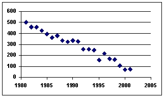
A)quadratic
B)cosine
C)linear
D)tangential
E)flat
A)quadratic
B)cosine
C)linear
D)tangential
E)flat
Question
Using a three-month moving average (with weights of 6,3,and 1 for the most current value,next most current value and oldest value,respectively),the forecast value for October made at the end of September in the following time series would be___. 
A)11.60
B)10.00
C)9.67
D)8.60
E)6.11
A)11.60
B)10.00
C)9.67
D)8.60
E)6.11
Question
Question
The following graph of a time-series data suggests a ___ trend. 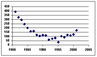
A)linear
B)tangential
C)cosine
D)quadratic
E)flat
A)linear
B)tangential
C)cosine
D)quadratic
E)flat
Question
Fitting a linear trend to 36 monthly data points (January 2000 = 1,February 2000 = 2,March 2000 = 3,etc. )produced the following tables: 
 The projected trend value for January 2003 is ___.
A)231.39
B)555.71
C)339.50
D)447.76
E)355.71
The projected trend value for January 2003 is ___.A)231.39
B)555.71
C)339.50
D)447.76
E)355.71
Question
The following graph of time-series data suggests a ___ trend. 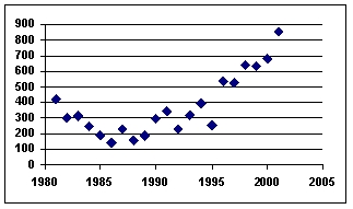
A)linear
B)quadratic
C)cosine
D)tangential
E)flat
A)linear
B)quadratic
C)cosine
D)tangential
E)flat
Question
Question
Question
Question
Analysis of data for an autoregressive forecasting model produced the following tables: 
 The forecasting model is ___.
A)yt = 5.745787 + 0.062849 yt-1 + 0.065709 yt-2
B)yt = 4.85094 - 0.10434 yt-1 + 0.962669 yt-2
C)yt = 0.84426 - 1.66023 yt-1 + 14.65023 yt-2
D)yt = 0.40299 + 0.103822 yt-1 + 9.yt-2
E)yt = 0.40299 + 0.103822 yt-1 - 9.yt-2
The forecasting model is ___.A)yt = 5.745787 + 0.062849 yt-1 + 0.065709 yt-2
B)yt = 4.85094 - 0.10434 yt-1 + 0.962669 yt-2
C)yt = 0.84426 - 1.66023 yt-1 + 14.65023 yt-2
D)yt = 0.40299 + 0.103822 yt-1 + 9.yt-2
E)yt = 0.40299 + 0.103822 yt-1 - 9.yt-2
Question
Fitting a linear trend to 36 monthly data points (January 2000 = 1,February 2000 = 2,March 2000 = 3,etc. )produced the following tables: 
 The projected trend value for January 2003 is ___.
A)544.29
B)868.61
C)652.39
D)760.50
E)876.90
The projected trend value for January 2003 is ___.A)544.29
B)868.61
C)652.39
D)760.50
E)876.90
Question
Question
The ratios of "actuals to moving averages" (seasonal indexes)for a time series are presented in the following table as percentages:  The final (completely adjusted)estimate of the seasonal index for Q1 is ___.
A)109.733
B)109.921
C)113.853
D)113.492
E)111.545
The final (completely adjusted)estimate of the seasonal index for Q1 is ___.A)109.733
B)109.921
C)113.853
D)113.492
E)111.545
Question
The ratios of "actuals to moving averages" (seasonal indexes)for a time series are presented in the following table as percentages:  The initial estimate of the seasonal index for Q1 is ___.
A)111.047
B)111.741
C)111.523
D)111.243
E)111.943
The initial estimate of the seasonal index for Q1 is ___.A)111.047
B)111.741
C)111.523
D)111.243
E)111.943
Question
The following graph of a time-series data suggests a ___ trend. 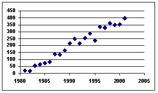
A)linear
B)quadratic
C)cosine
D)tangential
E)flat
A)linear
B)quadratic
C)cosine
D)tangential
E)flat
Question
Using a three-month moving average (with weights of 6,3,and 1 for the most current value,next most current value and oldest value,respectively),the forecast value for November in the following time series is ___. 
A)11.60
B)10.00
C)9.67
D)8.06
E)8.60
A)11.60
B)10.00
C)9.67
D)8.06
E)8.60
Question
Using 2000 as the base year,the 1990 value of the Paasche' Price Index is ___.(Quantities are averages for the student body. ) 
A)80.72
B)162.28
C)240.06
D)50.45
E)30.35
A)80.72
B)162.28
C)240.06
D)50.45
E)30.35
Question
Using 2008 as the base year,the 2007 value of the Paasche' Price Index is ___. 
A)99.79
B)192.51
C)100.29
D)59.19
E)39.99
A)99.79
B)192.51
C)100.29
D)59.19
E)39.99
Question
Question
Question
Jim Royo,manager of Billings Building Supply (BBS),wants to develop a model to forecast BBS's monthly sales (in $1,000's).He selects the dollar value of residential building permits (in $10,000)as the predictor variable.An analysis of the data yielded the following tables: 

Jim's calculated value for the Durbin-Watson statistic is 1.93.Using = 0.05,the appropriate decision is: ___.
A)do not reject H0: = 0
B)reject H0: ≠ 00
C)do not reject: 0
D)the test is inconclusive
E)reject H0: = 0
Jim's calculated value for the Durbin-Watson statistic is 1.93.Using = 0.05,the appropriate decision is: ___.
A)do not reject H0: = 0
B)reject H0: ≠ 00
C)do not reject: 0
D)the test is inconclusive
E)reject H0: = 0
Question
Using 2006 as the base year,the 2008 value of a simple price index for the following price data is ___. 
A)77.60
B)114.13
C)160.58
D)99.30
E)100.00
A)77.60
B)114.13
C)160.58
D)99.30
E)100.00
Question
Jim Royo,manager of Billings Building Supply (BBS),wants to develop a model to forecast BBS's monthly sales (in $1,000's).He selects the dollar value of residential building permits (in $10,000)as the predictor variable.An analysis of the data yielded the following tables: 

Using = 0.05 the critical value of the Durbin-Watson statistic,dU, is ___.
A)1.54
B)1.42
C)1.43
D)1.44
E)1.85
Using = 0.05 the critical value of the Durbin-Watson statistic,dU, is ___.
A)1.54
B)1.42
C)1.43
D)1.44
E)1.85
Question
Analysis of data for an autoregressive forecasting model produced the following tables: 
 The results indicate that ___.
A)the first predictor,yt-1,is significant at the 5% level
B)the second predictor,yt-2,is significant at the 5% level
C)all predictor variables are significant at the 5% level
D)none of the predictor variables are significant at the 5% level
E)the overall regression model is not significant at 5% level
The results indicate that ___.A)the first predictor,yt-1,is significant at the 5% level
B)the second predictor,yt-2,is significant at the 5% level
C)all predictor variables are significant at the 5% level
D)none of the predictor variables are significant at the 5% level
E)the overall regression model is not significant at 5% level
Question
Jim Royo,manager of Billings Building Supply (BBS),wants to develop a model to forecast BBS's monthly sales (in $1,000's).He selects the dollar value of residential building permits (in $10,000)as the predictor variable.An analysis of the data yielded the following tables: 

Using = 0.05 the critical value of the Durbin-Watson statistic,dL, is ___.
A)1.24
B)1.22
C)1.13
D)1.15
E)1.85
Using = 0.05 the critical value of the Durbin-Watson statistic,dL, is ___.
A)1.24
B)1.22
C)1.13
D)1.15
E)1.85
Question
Using 2008 as the base year,the 2007 value of the Laspeyres Price Index is ___. 
A)69.92
B)144.06
C)100.21
D)79.72
E)99.72
A)69.92
B)144.06
C)100.21
D)79.72
E)99.72
Question
Analysis of data for an autoregressive forecasting model produced the following tables: 
 The actual values of this time series,y,were 228,54,and 191 for May,June,and July,respectively.The predicted (forecast)value for August is ___.
A)174.41
B)83.67
C)218.71
D)36.91
E)191
The actual values of this time series,y,were 228,54,and 191 for May,June,and July,respectively.The predicted (forecast)value for August is ___.A)174.41
B)83.67
C)218.71
D)36.91
E)191
Question
Analysis of data for an autoregressive forecasting model produced the following tables: 
 The actual values of this time series,y,were 228,54,and 191 for May,June,and July,respectively.The forecast value predicted by the model for July is ___.
A)36.91
B)83.67
C)218.71
D)174.41
E)191
The actual values of this time series,y,were 228,54,and 191 for May,June,and July,respectively.The forecast value predicted by the model for July is ___.A)36.91
B)83.67
C)218.71
D)174.41
E)191
Question
Jim Royo,manager of Billings Building Supply (BBS),wants to develop a model to forecast BBS's monthly sales (in $1,000's).He selects the dollar value of residential building permits (in $10,000)as the predictor variable.An analysis of the data yielded the following tables: 

Jim's calculated value for the Durbin-Watson statistic is 1.14.Using = 0.05,the appropriate decision is: ___.
A)do not reject H0: = 0
B)reject H0: = 0
C)do not reject H0: 0
D)the test is inconclusive
E)reject H0: ≠ 0
Jim's calculated value for the Durbin-Watson statistic is 1.14.Using = 0.05,the appropriate decision is: ___.
A)do not reject H0: = 0
B)reject H0: = 0
C)do not reject H0: 0
D)the test is inconclusive
E)reject H0: ≠ 0
Question
Question
Question
Question

Unlock Deck
Sign up to unlock the cards in this deck!
Unlock Deck
Unlock Deck
1/77
Play
Full screen (f)
Deck 15: Time-Series Forecasting and Index Numbers
1
One of the main techniques for isolating the effects of seasonality is reconstitution.
False
2
When a trucking firm uses the number of shipments for January of the previous year as the forecast for January next year,it is using a naïve forecasting model.
True
3
Describe smoothing techniques for forecasting models,including naive,simple average,moving average,weighted moving average,and exponential smoothing.
One group of time-series forecasting methods contains smoothing techniques.Among these techniques are naïve models,averaging techniques,and simple exponential smoothing.These techniques do much better if the time-series data are stationary or show no significant trend or seasonal effects.Naive forecasting models are models in which it is assumed that the more recent time periods of data represent the best predictions or forecasts for future outcomes.
Simple averages use the average value for some given length of previous time periods to forecast the value for the next period.
Moving averages are time period averages that are revised for each time period by including the most recent value(s)in the computation of the average and deleting the value or values that are farthest away from the present time period.A special case of the moving average is the weighted moving average,in which different weights are placed on the values from different time periods.
Simple (single)exponential smoothing is a technique in which data from previous time periods are weighted exponentially to forecast the value for the present time period.The forecaster can select how much to weight more recent values versus those of previous time periods.
4
Because seasonal effects can confound trend analysis,it is important to make sure that the data is free of seasonality prior to using regression models to analyze trend.
Unlock Deck
Unlock for access to all 77 flashcards in this deck.
Unlock Deck
k this deck
5
Forecast error is the difference between the value of the response variable and those of the explanatory variables.
Unlock Deck
Unlock for access to all 77 flashcards in this deck.
Unlock Deck
k this deck
6
Differentiate among various measurements of forecasting error,including mean absolute deviation and mean square error,in order to assess which forecasting method to use.
Unlock Deck
Unlock for access to all 77 flashcards in this deck.
Unlock Deck
k this deck
7
Two popular general categories of smoothing techniques are averaging models and exponential models.
Unlock Deck
Unlock for access to all 77 flashcards in this deck.
Unlock Deck
k this deck
8
An exponential smoothing technique in which the smoothing constant alpha is equal to one is equivalent to a naïve forecasting model.
Unlock Deck
Unlock for access to all 77 flashcards in this deck.
Unlock Deck
k this deck
9
Test for autocorrelation using the Durbin-Watson test,overcoming it by adding independent variables and transforming variables and taking advantage of it with autoregression.
Unlock Deck
Unlock for access to all 77 flashcards in this deck.
Unlock Deck
k this deck
10
Account for seasonal effects of time-series data by using decomposition and Winters' three-parameter exponential smoothing method.
Unlock Deck
Unlock for access to all 77 flashcards in this deck.
Unlock Deck
k this deck
11
Linear regression models cannot be used to analyze quadratic trends in time-series data.
Unlock Deck
Unlock for access to all 77 flashcards in this deck.
Unlock Deck
k this deck
12
Differentiate among simple index numbers,unweighted aggregate price index numbers,weighted aggregate price index numbers,Laspeyres price index numbers,and Paasche price index numbers by defining and calculating each.
Unlock Deck
Unlock for access to all 77 flashcards in this deck.
Unlock Deck
k this deck
13
Two popular general categories of smoothing techniques are exponential models and logarithmic models.
Unlock Deck
Unlock for access to all 77 flashcards in this deck.
Unlock Deck
k this deck
14
The long-term general direction of data is referred to as trend.
Unlock Deck
Unlock for access to all 77 flashcards in this deck.
Unlock Deck
k this deck
15
Determine trend in time-series data by using linear regression trend analysis,quadratic model trend analysis,and Holt's two-parameter exponential smoothing method.
Unlock Deck
Unlock for access to all 77 flashcards in this deck.
Unlock Deck
k this deck
16
One of the main techniques for isolating the effects of seasonality is decomposition.
Unlock Deck
Unlock for access to all 77 flashcards in this deck.
Unlock Deck
k this deck
17
Mean error (ME)and mean absolute deviation (MAD)will have the same numerical value if all errors are positive.
Unlock Deck
Unlock for access to all 77 flashcards in this deck.
Unlock Deck
k this deck
18
Naïve forecasting models have no useful applications because they do not take into account data trend,cyclical effects or seasonality.
Unlock Deck
Unlock for access to all 77 flashcards in this deck.
Unlock Deck
k this deck
19
Time-series data are data gathered on a desired characteristic at a particular point in time.
Unlock Deck
Unlock for access to all 77 flashcards in this deck.
Unlock Deck
k this deck
20
A stationary time-series data has only trend but no cyclical or seasonal effects.
Unlock Deck
Unlock for access to all 77 flashcards in this deck.
Unlock Deck
k this deck
21
A time series with forecast values and error terms is presented in the following table.The mean squared error (MSE)for this forecast is ___.
A)13.33
B)17.94
C)89.71
D)22.42
E)32.34
A)13.33
B)17.94
C)89.71
D)22.42
E)32.34
Unlock Deck
Unlock for access to all 77 flashcards in this deck.
Unlock Deck
k this deck
22
If autocorrelation occurs in regression analysis,then the confidence intervals and tests using the t and F distributions are no longer strictly applicable.
Unlock Deck
Unlock for access to all 77 flashcards in this deck.
Unlock Deck
k this deck
23
A time series with forecast values and error terms is presented in the following table.The mean error (ME)for this forecast is ___.
A)-0.80
B)-1.00
C)-4.00
D)8.00
E)1.00
A)-0.80
B)-1.00
C)-4.00
D)8.00
E)1.00
Unlock Deck
Unlock for access to all 77 flashcards in this deck.
Unlock Deck
k this deck
24
In exponential smoothing models,the value of the smoothing constant may be any number between ___.
A)-1 and 1
B)-5 and 5
C)0 and 1
D)0 and 10
E)0 and 100
A)-1 and 1
B)-5 and 5
C)0 and 1
D)0 and 10
E)0 and 100
Unlock Deck
Unlock for access to all 77 flashcards in this deck.
Unlock Deck
k this deck
25
A time series with forecast values and error terms is presented in the following table.The mean squared error (MSE)for this forecast is ___.
A)8.86
B)44.31
C)3.28
D)11.08
E)28.01
A)8.86
B)44.31
C)3.28
D)11.08
E)28.01
Unlock Deck
Unlock for access to all 77 flashcards in this deck.
Unlock Deck
k this deck
26
Autoregression is a multiple regression technique in which the independent variables are time-lagged versions of the dependent variable.
Unlock Deck
Unlock for access to all 77 flashcards in this deck.
Unlock Deck
k this deck
27
A time series with forecast values and error terms is presented in the following table.The mean absolute deviation (MAD)for this forecast is ___.
A)3.54
B)7.41
C)4.43
D)17.72
E)4.34
A)3.54
B)7.41
C)4.43
D)17.72
E)4.34
Unlock Deck
Unlock for access to all 77 flashcards in this deck.
Unlock Deck
k this deck
28
A time series with forecast values and error terms is presented in the following table.The mean error (ME)for this forecast is ___.
A)1.67
B)1.34
C)6.68
D)3.67
E)2.87
A)1.67
B)1.34
C)6.68
D)3.67
E)2.87
Unlock Deck
Unlock for access to all 77 flashcards in this deck.
Unlock Deck
k this deck
29
Autocorrelation in a regression forecasting model can be detected by the F test.
Unlock Deck
Unlock for access to all 77 flashcards in this deck.
Unlock Deck
k this deck
30
Use of a smoothing constant value less than 0.5 in an exponential smoothing model gives more weight to ___.
A)the actual value for the current period
B)the actual value for the previous period
C)the forecast for the current period
D)the forecast for the previous period
E)the forecast for the next period
A)the actual value for the current period
B)the actual value for the previous period
C)the forecast for the current period
D)the forecast for the previous period
E)the forecast for the next period
Unlock Deck
Unlock for access to all 77 flashcards in this deck.
Unlock Deck
k this deck
31
One of the ways to overcome the autocorrelation problem in a regression forecasting model is to increase the level of significance for the F test
Unlock Deck
Unlock for access to all 77 flashcards in this deck.
Unlock Deck
k this deck
32
A time series with forecast values and error terms is presented in the following table.The mean absolute deviation (MAD)for this forecast is ___.
A)3.10
B)12.40
C)2.48
D)6.67
E)5.10
A)3.10
B)12.40
C)2.48
D)6.67
E)5.10
Unlock Deck
Unlock for access to all 77 flashcards in this deck.
Unlock Deck
k this deck
33
Using a three-month moving average,the forecast value for November in the following time series would be ___.
A)7.67
B)8
C)9
D)6.89
E)11.00
A)7.67
B)8
C)9
D)6.89
E)11.00
Unlock Deck
Unlock for access to all 77 flashcards in this deck.
Unlock Deck
k this deck
34
Using a three-month moving average (with weights of 5,3,and 1 for the most current value,next most current value and oldest value,respectively),the forecast value for November in the following time series would be ___.
A)7.67
B)8
C)9
D)6.89
E)11
A)7.67
B)8
C)9
D)6.89
E)11
Unlock Deck
Unlock for access to all 77 flashcards in this deck.
Unlock Deck
k this deck
35
When forecasting with exponential smoothing,data from previous periods is ___.
A)given equal importance
B)given exponentially increasing importance
C)ignored
D)given exponentially decreasing importance
E)linearly decreasing importance
A)given equal importance
B)given exponentially increasing importance
C)ignored
D)given exponentially decreasing importance
E)linearly decreasing importance
Unlock Deck
Unlock for access to all 77 flashcards in this deck.
Unlock Deck
k this deck
36
Using a three-month moving average (with weights of 5,3,and 1 for the most current value,next most current value and oldest value,respectively),the forecast value for October made at the end of September in the following time series would be ___.
A)7.67
B)8
C)9
D)6.89
E)11
A)7.67
B)8
C)9
D)6.89
E)11
Unlock Deck
Unlock for access to all 77 flashcards in this deck.
Unlock Deck
k this deck
37
Using a three-month moving average,the forecast value for October made at the end of September in the following time series would be ___.
A)7.67
B)8
C)9
D)6.89
E)7.25
A)7.67
B)8
C)9
D)6.89
E)7.25
Unlock Deck
Unlock for access to all 77 flashcards in this deck.
Unlock Deck
k this deck
38
One of the ways to overcome the autocorrelation problem in a regression forecasting model is to transform the variables by taking the first-order differences.
Unlock Deck
Unlock for access to all 77 flashcards in this deck.
Unlock Deck
k this deck
39
Use of a smoothing constant value greater than 0.5 in an exponential smoothing model gives more weight to ___.
A)the actual value for the current period
B)the actual value for the previous period
C)the forecast for the current period
D)the forecast for the previous period
E)the forecast for the next period
A)the actual value for the current period
B)the actual value for the previous period
C)the forecast for the current period
D)the forecast for the previous period
E)the forecast for the next period
Unlock Deck
Unlock for access to all 77 flashcards in this deck.
Unlock Deck
k this deck
40
When the error terms of a regression forecasting model are correlated the problem of multicollinearity occurs.
Unlock Deck
Unlock for access to all 77 flashcards in this deck.
Unlock Deck
k this deck
41
Using a three-month moving average,the forecast value for November in the following time series is ___.
A)11.60
B)10.00
C)9.67
D)8.60
E)6.00
A)11.60
B)10.00
C)9.67
D)8.60
E)6.00
Unlock Deck
Unlock for access to all 77 flashcards in this deck.
Unlock Deck
k this deck
42
Using a three-month moving average,the forecast value for October made at the end of September in the following time series would be ___.
A)11.60
B)10.00
C)9.07
D)8.06
E)9.67
A)11.60
B)10.00
C)9.07
D)8.06
E)9.67
Unlock Deck
Unlock for access to all 77 flashcards in this deck.
Unlock Deck
k this deck
43
What is the forecast for the Period 7 using a 3-period moving average technique,given the following time-series data for six past periods?
A)164.67
B)156.00
C)148.00
D)126.57
E)158.67
A)164.67
B)156.00
C)148.00
D)126.57
E)158.67
Unlock Deck
Unlock for access to all 77 flashcards in this deck.
Unlock Deck
k this deck
44
The high and low values of the "ratios of actuals to moving average" are ignored when finalizing the seasonal index for a period (month or quarter)in time series decomposition.The rationale for this is to ___.
A)reduce the sample size
B)eliminate autocorrelation
C)minimize serial correlation
D)eliminate the irregular component
E)eliminate the trend
A)reduce the sample size
B)eliminate autocorrelation
C)minimize serial correlation
D)eliminate the irregular component
E)eliminate the trend
Unlock Deck
Unlock for access to all 77 flashcards in this deck.
Unlock Deck
k this deck
45
The following graph of time-series data suggests a ___ trend.
A)quadratic
B)cosine
C)linear
D)tangential
E)flat
A)quadratic
B)cosine
C)linear
D)tangential
E)flat
Unlock Deck
Unlock for access to all 77 flashcards in this deck.
Unlock Deck
k this deck
46
Using a three-month moving average (with weights of 6,3,and 1 for the most current value,next most current value and oldest value,respectively),the forecast value for October made at the end of September in the following time series would be___.
A)11.60
B)10.00
C)9.67
D)8.60
E)6.11
A)11.60
B)10.00
C)9.67
D)8.60
E)6.11
Unlock Deck
Unlock for access to all 77 flashcards in this deck.
Unlock Deck
k this deck
47
Calculating the "ratios of actuals to moving average" is a common step in time series decomposition.The results (the quotients)of this step estimate the ___.
A)trend and cyclical components
B)seasonal and irregular components
C)cyclical and irregular components
D)trend and seasonal components
E)irregular components
A)trend and cyclical components
B)seasonal and irregular components
C)cyclical and irregular components
D)trend and seasonal components
E)irregular components
Unlock Deck
Unlock for access to all 77 flashcards in this deck.
Unlock Deck
k this deck
48
The following graph of a time-series data suggests a ___ trend.
A)linear
B)tangential
C)cosine
D)quadratic
E)flat
A)linear
B)tangential
C)cosine
D)quadratic
E)flat
Unlock Deck
Unlock for access to all 77 flashcards in this deck.
Unlock Deck
k this deck
49
Fitting a linear trend to 36 monthly data points (January 2000 = 1,February 2000 = 2,March 2000 = 3,etc. )produced the following tables: The projected trend value for January 2003 is ___.
A)231.39
B)555.71
C)339.50
D)447.76
E)355.71
The projected trend value for January 2003 is ___.A)231.39
B)555.71
C)339.50
D)447.76
E)355.71
Unlock Deck
Unlock for access to all 77 flashcards in this deck.
Unlock Deck
k this deck
50
The following graph of time-series data suggests a ___ trend.
A)linear
B)quadratic
C)cosine
D)tangential
E)flat
A)linear
B)quadratic
C)cosine
D)tangential
E)flat
Unlock Deck
Unlock for access to all 77 flashcards in this deck.
Unlock Deck
k this deck
51
The forecast value for August was 12 and the actual value turned out to be 5.Using exponential smoothing with = 0.20,the forecast value for September would be ___.
A)10.10
B)9.88
C)12.00
D)10.6
E)11
A)10.10
B)9.88
C)12.00
D)10.6
E)11
Unlock Deck
Unlock for access to all 77 flashcards in this deck.
Unlock Deck
k this deck
52
In an autoregressive forecasting model,the independent variable(s)is (are)___.
A)time-lagged values of the dependent variable
B)first-order differences of the dependent variable
C)second-order,or higher,differences of the dependent variable
D)first-order quotients of the dependent variable
E)time-lagged values of the independent variable
A)time-lagged values of the dependent variable
B)first-order differences of the dependent variable
C)second-order,or higher,differences of the dependent variable
D)first-order quotients of the dependent variable
E)time-lagged values of the independent variable
Unlock Deck
Unlock for access to all 77 flashcards in this deck.
Unlock Deck
k this deck
53
Which of the following is not a component of time series data?
A)trend
B)seasonal fluctuations
C)cyclical fluctuations
D)normal fluctuations
E)irregular fluctuations
A)trend
B)seasonal fluctuations
C)cyclical fluctuations
D)normal fluctuations
E)irregular fluctuations
Unlock Deck
Unlock for access to all 77 flashcards in this deck.
Unlock Deck
k this deck
54
Analysis of data for an autoregressive forecasting model produced the following tables: The forecasting model is ___.
A)yt = 5.745787 + 0.062849 yt-1 + 0.065709 yt-2
B)yt = 4.85094 - 0.10434 yt-1 + 0.962669 yt-2
C)yt = 0.84426 - 1.66023 yt-1 + 14.65023 yt-2
D)yt = 0.40299 + 0.103822 yt-1 + 9.yt-2
E)yt = 0.40299 + 0.103822 yt-1 - 9.yt-2
The forecasting model is ___.A)yt = 5.745787 + 0.062849 yt-1 + 0.065709 yt-2
B)yt = 4.85094 - 0.10434 yt-1 + 0.962669 yt-2
C)yt = 0.84426 - 1.66023 yt-1 + 14.65023 yt-2
D)yt = 0.40299 + 0.103822 yt-1 + 9.yt-2
E)yt = 0.40299 + 0.103822 yt-1 - 9.yt-2
Unlock Deck
Unlock for access to all 77 flashcards in this deck.
Unlock Deck
k this deck
55
Fitting a linear trend to 36 monthly data points (January 2000 = 1,February 2000 = 2,March 2000 = 3,etc. )produced the following tables: The projected trend value for January 2003 is ___.
A)544.29
B)868.61
C)652.39
D)760.50
E)876.90
The projected trend value for January 2003 is ___.A)544.29
B)868.61
C)652.39
D)760.50
E)876.90
Unlock Deck
Unlock for access to all 77 flashcards in this deck.
Unlock Deck
k this deck
56
The forecast value for September was 10.6 and the actual value turned out to be 7.Using exponential smoothing with = 0.20,the forecast value for October would be ___.
A)10.10
B)9.88
C)12.00
D)10.6
E)8.88
A)10.10
B)9.88
C)12.00
D)10.6
E)8.88
Unlock Deck
Unlock for access to all 77 flashcards in this deck.
Unlock Deck
k this deck
57
The ratios of "actuals to moving averages" (seasonal indexes)for a time series are presented in the following table as percentages: The final (completely adjusted)estimate of the seasonal index for Q1 is ___.
A)109.733
B)109.921
C)113.853
D)113.492
E)111.545
The final (completely adjusted)estimate of the seasonal index for Q1 is ___.A)109.733
B)109.921
C)113.853
D)113.492
E)111.545
Unlock Deck
Unlock for access to all 77 flashcards in this deck.
Unlock Deck
k this deck
58
The ratios of "actuals to moving averages" (seasonal indexes)for a time series are presented in the following table as percentages: The initial estimate of the seasonal index for Q1 is ___.
A)111.047
B)111.741
C)111.523
D)111.243
E)111.943
The initial estimate of the seasonal index for Q1 is ___.A)111.047
B)111.741
C)111.523
D)111.243
E)111.943
Unlock Deck
Unlock for access to all 77 flashcards in this deck.
Unlock Deck
k this deck
59
The following graph of a time-series data suggests a ___ trend.
A)linear
B)quadratic
C)cosine
D)tangential
E)flat
A)linear
B)quadratic
C)cosine
D)tangential
E)flat
Unlock Deck
Unlock for access to all 77 flashcards in this deck.
Unlock Deck
k this deck
60
Using a three-month moving average (with weights of 6,3,and 1 for the most current value,next most current value and oldest value,respectively),the forecast value for November in the following time series is ___.
A)11.60
B)10.00
C)9.67
D)8.06
E)8.60
A)11.60
B)10.00
C)9.67
D)8.06
E)8.60
Unlock Deck
Unlock for access to all 77 flashcards in this deck.
Unlock Deck
k this deck
61
Using 2000 as the base year,the 1990 value of the Paasche' Price Index is ___.(Quantities are averages for the student body. )
A)80.72
B)162.28
C)240.06
D)50.45
E)30.35
A)80.72
B)162.28
C)240.06
D)50.45
E)30.35
Unlock Deck
Unlock for access to all 77 flashcards in this deck.
Unlock Deck
k this deck
62
Using 2008 as the base year,the 2007 value of the Paasche' Price Index is ___.
A)99.79
B)192.51
C)100.29
D)59.19
E)39.99
A)99.79
B)192.51
C)100.29
D)59.19
E)39.99
Unlock Deck
Unlock for access to all 77 flashcards in this deck.
Unlock Deck
k this deck
63
The motivation for using an index number is to ___.
A)transform the data to a standard normal distribution
B)transform the data for a linear model
C)eliminate bias from the sample
D)reduce data to an easier-to-use,more convenient form
E)reduce the variance in the data
A)transform the data to a standard normal distribution
B)transform the data for a linear model
C)eliminate bias from the sample
D)reduce data to an easier-to-use,more convenient form
E)reduce the variance in the data
Unlock Deck
Unlock for access to all 77 flashcards in this deck.
Unlock Deck
k this deck
64
Index numbers facilitate comparison of ___.
A)means
B)data over time
C)variances
D)samples
E)deviations
A)means
B)data over time
C)variances
D)samples
E)deviations
Unlock Deck
Unlock for access to all 77 flashcards in this deck.
Unlock Deck
k this deck
65
Jim Royo,manager of Billings Building Supply (BBS),wants to develop a model to forecast BBS's monthly sales (in $1,000's).He selects the dollar value of residential building permits (in $10,000)as the predictor variable.An analysis of the data yielded the following tables:
Jim's calculated value for the Durbin-Watson statistic is 1.93.Using = 0.05,the appropriate decision is: ___.
A)do not reject H0: = 0
B)reject H0: ≠ 00
C)do not reject: 0
D)the test is inconclusive
E)reject H0: = 0
Jim's calculated value for the Durbin-Watson statistic is 1.93.Using = 0.05,the appropriate decision is: ___.
A)do not reject H0: = 0
B)reject H0: ≠ 00
C)do not reject: 0
D)the test is inconclusive
E)reject H0: = 0
Unlock Deck
Unlock for access to all 77 flashcards in this deck.
Unlock Deck
k this deck
66
Using 2006 as the base year,the 2008 value of a simple price index for the following price data is ___.
A)77.60
B)114.13
C)160.58
D)99.30
E)100.00
A)77.60
B)114.13
C)160.58
D)99.30
E)100.00
Unlock Deck
Unlock for access to all 77 flashcards in this deck.
Unlock Deck
k this deck
67
Jim Royo,manager of Billings Building Supply (BBS),wants to develop a model to forecast BBS's monthly sales (in $1,000's).He selects the dollar value of residential building permits (in $10,000)as the predictor variable.An analysis of the data yielded the following tables:
Using = 0.05 the critical value of the Durbin-Watson statistic,dU, is ___.
A)1.54
B)1.42
C)1.43
D)1.44
E)1.85
Using = 0.05 the critical value of the Durbin-Watson statistic,dU, is ___.
A)1.54
B)1.42
C)1.43
D)1.44
E)1.85
Unlock Deck
Unlock for access to all 77 flashcards in this deck.
Unlock Deck
k this deck
68
Analysis of data for an autoregressive forecasting model produced the following tables: The results indicate that ___.
A)the first predictor,yt-1,is significant at the 5% level
B)the second predictor,yt-2,is significant at the 5% level
C)all predictor variables are significant at the 5% level
D)none of the predictor variables are significant at the 5% level
E)the overall regression model is not significant at 5% level
The results indicate that ___.A)the first predictor,yt-1,is significant at the 5% level
B)the second predictor,yt-2,is significant at the 5% level
C)all predictor variables are significant at the 5% level
D)none of the predictor variables are significant at the 5% level
E)the overall regression model is not significant at 5% level
Unlock Deck
Unlock for access to all 77 flashcards in this deck.
Unlock Deck
k this deck
69
Jim Royo,manager of Billings Building Supply (BBS),wants to develop a model to forecast BBS's monthly sales (in $1,000's).He selects the dollar value of residential building permits (in $10,000)as the predictor variable.An analysis of the data yielded the following tables:
Using = 0.05 the critical value of the Durbin-Watson statistic,dL, is ___.
A)1.24
B)1.22
C)1.13
D)1.15
E)1.85
Using = 0.05 the critical value of the Durbin-Watson statistic,dL, is ___.
A)1.24
B)1.22
C)1.13
D)1.15
E)1.85
Unlock Deck
Unlock for access to all 77 flashcards in this deck.
Unlock Deck
k this deck
70
Using 2008 as the base year,the 2007 value of the Laspeyres Price Index is ___.
A)69.92
B)144.06
C)100.21
D)79.72
E)99.72
A)69.92
B)144.06
C)100.21
D)79.72
E)99.72
Unlock Deck
Unlock for access to all 77 flashcards in this deck.
Unlock Deck
k this deck
71
Analysis of data for an autoregressive forecasting model produced the following tables: The actual values of this time series,y,were 228,54,and 191 for May,June,and July,respectively.The predicted (forecast)value for August is ___.
A)174.41
B)83.67
C)218.71
D)36.91
E)191
The actual values of this time series,y,were 228,54,and 191 for May,June,and July,respectively.The predicted (forecast)value for August is ___.A)174.41
B)83.67
C)218.71
D)36.91
E)191
Unlock Deck
Unlock for access to all 77 flashcards in this deck.
Unlock Deck
k this deck
72
Analysis of data for an autoregressive forecasting model produced the following tables: The actual values of this time series,y,were 228,54,and 191 for May,June,and July,respectively.The forecast value predicted by the model for July is ___.
A)36.91
B)83.67
C)218.71
D)174.41
E)191
The actual values of this time series,y,were 228,54,and 191 for May,June,and July,respectively.The forecast value predicted by the model for July is ___.A)36.91
B)83.67
C)218.71
D)174.41
E)191
Unlock Deck
Unlock for access to all 77 flashcards in this deck.
Unlock Deck
k this deck
73
Jim Royo,manager of Billings Building Supply (BBS),wants to develop a model to forecast BBS's monthly sales (in $1,000's).He selects the dollar value of residential building permits (in $10,000)as the predictor variable.An analysis of the data yielded the following tables:
Jim's calculated value for the Durbin-Watson statistic is 1.14.Using = 0.05,the appropriate decision is: ___.
A)do not reject H0: = 0
B)reject H0: = 0
C)do not reject H0: 0
D)the test is inconclusive
E)reject H0: ≠ 0
Jim's calculated value for the Durbin-Watson statistic is 1.14.Using = 0.05,the appropriate decision is: ___.
A)do not reject H0: = 0
B)reject H0: = 0
C)do not reject H0: 0
D)the test is inconclusive
E)reject H0: ≠ 0
Unlock Deck
Unlock for access to all 77 flashcards in this deck.
Unlock Deck
k this deck
74
When constructing a weighted aggregate price index,the weights usually are ___.
A)prices of substitute items
B)prices of complementary items
C)quantities of the respective items
D)squared quantities of the respective items
E)quality of individual items
A)prices of substitute items
B)prices of complementary items
C)quantities of the respective items
D)squared quantities of the respective items
E)quality of individual items
Unlock Deck
Unlock for access to all 77 flashcards in this deck.
Unlock Deck
k this deck
75
Typically,the denominator used to calculate an index number is a measurement for the ___ period.
A)base
B)current
C)spanning
D)intermediate
E)peak
A)base
B)current
C)spanning
D)intermediate
E)peak
Unlock Deck
Unlock for access to all 77 flashcards in this deck.
Unlock Deck
k this deck
76
Often,index numbers are expressed as ___.
A)percentages
B)frequencies
C)cycles
D)regression coefficients
E)correlation coefficients
A)percentages
B)frequencies
C)cycles
D)regression coefficients
E)correlation coefficients
Unlock Deck
Unlock for access to all 77 flashcards in this deck.
Unlock Deck
k this deck
77
Weighted aggregate price indexes are also known as ___.
A)unbalanced indexes
B)balanced indexes
C)value indexes
D)multiplicative indexes
E)overall indexes
A)unbalanced indexes
B)balanced indexes
C)value indexes
D)multiplicative indexes
E)overall indexes
Unlock Deck
Unlock for access to all 77 flashcards in this deck.
Unlock Deck
k this deck
Unlock Deck
Unlock for access to all 77 flashcards in this deck.


