Deck 22: Time Series Econometrics: Forecasting
Full screen (f)
Question
Question
Question
Question
Question
Question
Question
Question
Question
Question
Question
Question
Question
Question
Question
Question
Question
Question
Question
Question
Question
Question
Question
Continue with the data given in Table 17.5. Now consider the following simple model of money demand in Canada: 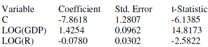
a. How would you interpret the parameters of this model
b. Obtain the residuals from this model and find out if there is any ARCH effect.
a. How would you interpret the parameters of this model
b. Obtain the residuals from this model and find out if there is any ARCH effect.
Question
Refer to the ARCH(2) model given in Eq. (22.11.4). Using the same data we estimated the following ARCH(1) model: 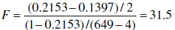

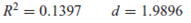
How would you choose between the two models Show the necessary calculations.
How would you choose between the two models Show the necessary calculations.
Question
Question
Question

Unlock Deck
Sign up to unlock the cards in this deck!
Unlock Deck
Unlock Deck
1/27
Play
Full screen (f)
Deck 22: Time Series Econometrics: Forecasting
1
What are the major methods of economic forecasting
Economic forecasting based on time series data is an essential field of econometric analysis. The major methods of economic forecasting are,
Exponential Smoothing Methods
In Exponential Smoothing methods, an appropriate curve based on the time series data is developed and used for economic forecasting in several areas of business.
Single-Equation Regression Models
In Single-Equation regression methods, an appropriate model is developed from the time series data. This model is used for forecasting the future values.
Simultaneous-Equation Regression Models
These models include more than one regression equation. Each mutually or jointly dependent economic variable has one equation. These models assume that there is two-way relationship among dependent and explanatory variables as an economic variable affects other economic variables and is also affected by them.
Autoregressive Integrated Moving Average (ARIMA) Models
ARIMA Models are also known as Box-Jenkins (BJ) methods. These models also include developing single or simultaneous equation models but unlike above models, these equations are not based on any economic theory but are created by analyzing properties of economic time series. In these models, the dependent variable is explained by lagged values of explanatory variables, lagged values of dependent variable itself, and stochastic error terms, in addition to explanatory variables.
Vector Autoregression (VAR) Models
VAR models are similar to simultaneous-equation models which consider more than one regression equation. But in VAR models, dependent variable is explained by lagged values of itself and lagged values of other explanatory endogenous variables. In VAR models, no variable is exogenous variable.
2
What are the major differences between simultaneous-equation and Box-Jenkins approaches to economic forecasting
Simultaneous equations approach includes more than one regression equation that is based on some economic theory. Each mutually or jointly dependent economic variable has one equation and together they explain any economic phenomenon.
Box-Jenkins (BJ) approach includes developing single or simultaneous equations but unlike simultaneous equations models, these equations are not based on any economic theory but are created by analyzing properties of economic time series.
Simultaneous equations approach assumes that there is two-way relationship among dependent and explanatory variables but it doesn't include lagged terms of explanatory and dependent variable.
Box-Jenkins (BJ) approach, in addition to explanatory variables, explains the dependent variable by lagged values of explanatory variables, lagged values of dependent variable itself, and stochastic error terms.
3
Outline the major steps involved in the application of the Box-Jenkins approach to forecasting.
Box-Jenkins (BJ) approach of economic forecasting includes developing single or simultaneous equations models, which are based on properties of economic time series rather than economic theory. This approach is popular in econometric analysis for its success in forecasting.
The method consists of four steps:
1. Identification.
The first step is identification of the model which involves finding number of autoregressive terms p , number of moving average terms q and integrated order term d.
2. Estimation.
The next step is estimation in which the parameters of the chosen model are estimated including the autoregressive and moving average terms.
3. Diagnostic checking.
In this step, it is checked whether the chosen model is the right model for the data. This is done by testing the residuals estimated from the chosen model, that they are white noise or not. If the residuals are white noise, the chosen mode is accepted for forecasting, otherwise another new model is developed and the first three steps are repeated again.
4. Forecasting.
The last step of Box-Jenkins (BJ) approach is forecasting the future values using the correct chosen model.
4
What happens if BoxJenkins techniques are applied to time series that are nonstationary
Unlock Deck
Unlock for access to all 27 flashcards in this deck.
Unlock Deck
k this deck
5
What are the differences between Box-Jenkins and VAR approaches to economic forecasting
Unlock Deck
Unlock for access to all 27 flashcards in this deck.
Unlock Deck
k this deck
6
In what sense is VAR atheoretic
Unlock Deck
Unlock for access to all 27 flashcards in this deck.
Unlock Deck
k this deck
7
"If the primary object is forecasting, VAR will do the job." Critically evaluate this statement.
Unlock Deck
Unlock for access to all 27 flashcards in this deck.
Unlock Deck
k this deck
8
Since the number of lags to be introduced in a VAR model can be a subjective question, how does one decide how many lags to introduce in a concrete application
Unlock Deck
Unlock for access to all 27 flashcards in this deck.
Unlock Deck
k this deck
9
Comment on this statement: "BoxJenkins and VAR are prime examples of measurement without theory."
Unlock Deck
Unlock for access to all 27 flashcards in this deck.
Unlock Deck
k this deck
10
What is the connection, if any, between Granger causality tests and VAR modeling
Unlock Deck
Unlock for access to all 27 flashcards in this deck.
Unlock Deck
k this deck
11
Consider the data on log DPI (personal disposable income) introduced in Section 21.1 (see the book's website for the actual data). Suppose you want to fit a suitable ARIMA model to these data. Outline the steps involved in carrying out this task.
Unlock Deck
Unlock for access to all 27 flashcards in this deck.
Unlock Deck
k this deck
12
Repeat Exercise 22.11 for the LPCE (personal consumption expenditure) data introduced in Section 21.1 (again, see the book's website for the actual data).
Unlock Deck
Unlock for access to all 27 flashcards in this deck.
Unlock Deck
k this deck
13
Repeat Exercise 22.11 for the LCP.
Unlock Deck
Unlock for access to all 27 flashcards in this deck.
Unlock Deck
k this deck
14
Repeat Exercise 22.11 for the LDNIDENDS.
Unlock Deck
Unlock for access to all 27 flashcards in this deck.
Unlock Deck
k this deck
15
In Section 13.9 you were introduced to the Schwarz Information criterion (SIC) to determine lag length. How would you use this criterion to determine the appropriate lag length in a VAR model
Unlock Deck
Unlock for access to all 27 flashcards in this deck.
Unlock Deck
k this deck
16
Using the data on LPCE and LDPI introduced in Section 21.1 (see the book's website for the actual data), develop a bivariate VAR model for the period 1970I to 2006IV. Use this model to forecast the values of these variables for the four quarters of 2007 and compare the forecast values with the actual values given in the dataset.
Unlock Deck
Unlock for access to all 27 flashcards in this deck.
Unlock Deck
k this deck
17
Repeat Exercise 22.16, using the data on LDIVIDENDS and LCP.
Unlock Deck
Unlock for access to all 27 flashcards in this deck.
Unlock Deck
k this deck
18
Refer to any statistical package and estimate the impulse response function for a period of up to 8 lags for the VAR model that you developed in Exercise 22.16.
Unlock Deck
Unlock for access to all 27 flashcards in this deck.
Unlock Deck
k this deck
19
Repeat Exercise 22.18 for the VAR model that you developed in Exercise 22.17.
Unlock Deck
Unlock for access to all 27 flashcards in this deck.
Unlock Deck
k this deck
20
Refer to the VAR regression results given in Table 22.4. From the various F tests reported in the three regressions given there, what can you say about the nature of causality in the three variables
Unlock Deck
Unlock for access to all 27 flashcards in this deck.
Unlock Deck
k this deck
21
Continuing with Exercise 20.20, can you guess why the authors chose to express the three variables in the model in percentage change form rather than using the levels of these variables ( Hint: Stationarity.)
Unlock Deck
Unlock for access to all 27 flashcards in this deck.
Unlock Deck
k this deck
22
Using the Canadian data given in Table 17.5, find out if M 1 and R are stationary random variables. If not, are they cointegrated Show the necessary calculations.
Unlock Deck
Unlock for access to all 27 flashcards in this deck.
Unlock Deck
k this deck
23
Continue with the data given in Table 17.5. Now consider the following simple model of money demand in Canada:
a. How would you interpret the parameters of this model
b. Obtain the residuals from this model and find out if there is any ARCH effect.
a. How would you interpret the parameters of this model
b. Obtain the residuals from this model and find out if there is any ARCH effect.
Unlock Deck
Unlock for access to all 27 flashcards in this deck.
Unlock Deck
k this deck
24
Refer to the ARCH(2) model given in Eq. (22.11.4). Using the same data we estimated the following ARCH(1) model:
How would you choose between the two models Show the necessary calculations.
How would you choose between the two models Show the necessary calculations.
Unlock Deck
Unlock for access to all 27 flashcards in this deck.
Unlock Deck
k this deck
25
Table 22.7 gives data on three-month (TB3M) and six-month (TB6M) Treasury bill rates from January 1, 1982, to March 2008, for a total of 315 monthly observations. The data can be found on the textbook's website.
a. Plot the two time series in the same diagram. What do you see
b. Do a formal unit root analysis to find out if these time series are stationary.
c. Are the two time series cointegrated How do you know Show the necessary calculations.
d. What is the economic meaning of cointegration in the present context If the two series are not cointegrated, what are the economic implications
e. If you want to estimate a VAR model, say, with four lags of each variable, do you have to use the first differences of the two series or can you do the analysis in levels of the two series Justify your answer.
Unlock Deck
Unlock for access to all 27 flashcards in this deck.
Unlock Deck
k this deck
26
Class Exercise: Pick a stock market index of your choosing and obtain daily data on the value of the chosen index for five years to find out if the stock index is characterized by ARCH effects.
Unlock Deck
Unlock for access to all 27 flashcards in this deck.
Unlock Deck
k this deck
27
Class Exercise: Collect data on inflation and unemployment rates in the U.S. for the quarterly periods in 1980-2007 and develop and estimate a VAR model for the two variables. To compute the inflation rate, use CPI (consumer price index) and use the civilian unemployment rate for the unemployment rate. Pay careful attention to the stationarity of these variables. Also, find out if one variable Granger-causes the other variable. Present all your calculations.
Unlock Deck
Unlock for access to all 27 flashcards in this deck.
Unlock Deck
k this deck
Unlock Deck
Unlock for access to all 27 flashcards in this deck.


