Deck 7: Inference When Variables Are Related
Full screen (f)
Question
Question
Homelessness is a problem in many large U.S. cities. To better understand the problem, a
multiple regression was used to model the rate of homelessness based on several
explanatory variables. The following data were collected for 50 large U.S. cities. The
regression results appear below.
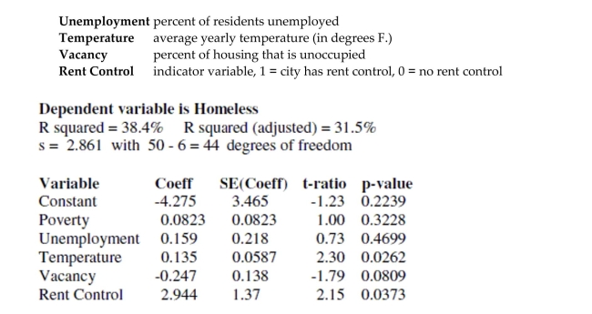
a. Using a 5% level of significance, which variables are associated with the number of
homeless in a city?
b. Explain the meaning of the coefficient of temperature in the context of this problem.
c. Explain the meaning of the coefficient of rent control in the context of this problem.
d. Do the results suggest that having rent control laws in a city causes higher levels of
homelessness? Explain.
e. If we created a new model by adding several more explanatory variables, which statistic
should be used to compare them - the R2 or the adjusted R2 ? Explain.
f. Using the plots below, check the regression conditions.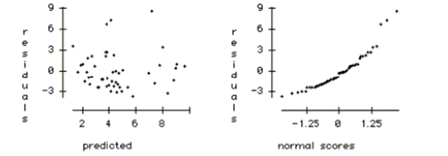
multiple regression was used to model the rate of homelessness based on several
explanatory variables. The following data were collected for 50 large U.S. cities. The
regression results appear below.
a. Using a 5% level of significance, which variables are associated with the number of
homeless in a city?
b. Explain the meaning of the coefficient of temperature in the context of this problem.
c. Explain the meaning of the coefficient of rent control in the context of this problem.
d. Do the results suggest that having rent control laws in a city causes higher levels of
homelessness? Explain.
e. If we created a new model by adding several more explanatory variables, which statistic
should be used to compare them - the R2 or the adjusted R2 ? Explain.
f. Using the plots below, check the regression conditions.
Question
Question
Question
Engineers want to know what factors are associated with gas mileage. The regression
below predicts the average miles per gallon (MPG) for 82 cars using their engine
horsepower (HP) and weight (WT, in 100's of pounds).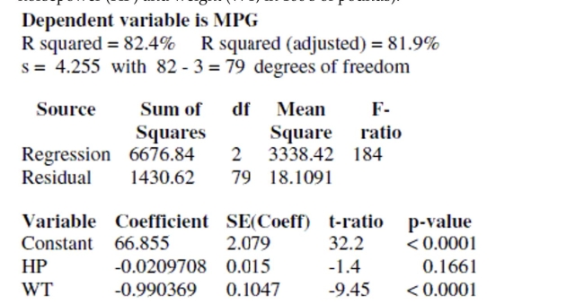
a. Write down the regression equation.
b. Write down the hypotheses for the test of the coefficient of horsepower. Conduct the test
and explain your conclusion in the context of this problem.
c. Write down the hypotheses for the test of the coefficient of weight. Conduct the test and
explain your conclusion in the context of this problem.
d. Explain the meaning of the coefficient of weight in the context of this problem.
e. Explain the meaning of the intercept of this regression in the context of this problem.
f. Compute the predicted gas mileage of a 3500 pound car with a 150 horsepower engine.
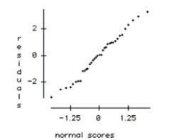
The plots are MPG vs. HP, MPG vs. WT, residuals vs. predicted values, and a normal
probability plot of residuals.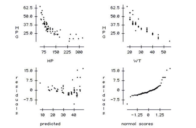
g. Check the conditions of this regression and comment on whether they are satisfied.
below predicts the average miles per gallon (MPG) for 82 cars using their engine
horsepower (HP) and weight (WT, in 100's of pounds).
a. Write down the regression equation.
b. Write down the hypotheses for the test of the coefficient of horsepower. Conduct the test
and explain your conclusion in the context of this problem.
c. Write down the hypotheses for the test of the coefficient of weight. Conduct the test and
explain your conclusion in the context of this problem.
d. Explain the meaning of the coefficient of weight in the context of this problem.
e. Explain the meaning of the intercept of this regression in the context of this problem.
f. Compute the predicted gas mileage of a 3500 pound car with a 150 horsepower engine.
The plots are MPG vs. HP, MPG vs. WT, residuals vs. predicted values, and a normal
probability plot of residuals.
g. Check the conditions of this regression and comment on whether they are satisfied.
Question
Here are data about the average January low temperature in cities in the United States, and factors that might allow us to
predict temperature. The data, available for 55 cities, include: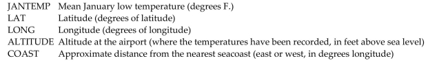 We will attempt to make a regression model to help account for mean January temperature and to understand the effects of
the various predictors.
At each step of the analysis you may assume that things learned earlier in the process are known.
Units Note: The "degrees" of temperature, given here on the Fahrenheit scale, have only coincidental language relationship to
the "degrees" of longitude and latitude. The geographic "degrees" are based on modeling the Earth as a sphere and dividing it
up into 360 degrees for a full circle. Thus 180 degrees of longitude is halfway around the world from Greenwich, England
(0°) and Latitude increases from 0 degrees at the Equator to 90 degrees of (North) latitude at the North Pole.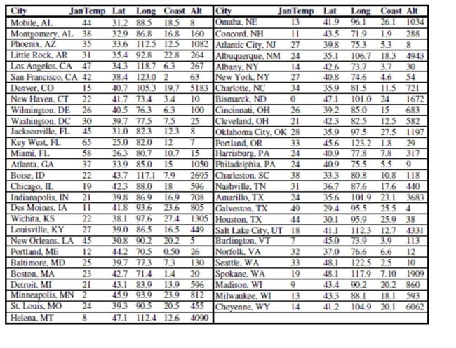
It is possible that the distance that a city is from the ocean could affect its average January
low temperature. Coast gives an approximate distance of each city from the East Coast or
West Coast (whichever is nearer). Including it in the regression yields the following
regression table: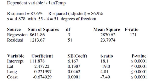
And here is a scatterplot of the residuals: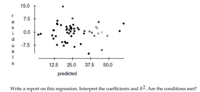
predict temperature. The data, available for 55 cities, include:
We will attempt to make a regression model to help account for mean January temperature and to understand the effects ofthe various predictors.
At each step of the analysis you may assume that things learned earlier in the process are known.
Units Note: The "degrees" of temperature, given here on the Fahrenheit scale, have only coincidental language relationship to
the "degrees" of longitude and latitude. The geographic "degrees" are based on modeling the Earth as a sphere and dividing it
up into 360 degrees for a full circle. Thus 180 degrees of longitude is halfway around the world from Greenwich, England
(0°) and Latitude increases from 0 degrees at the Equator to 90 degrees of (North) latitude at the North Pole.
It is possible that the distance that a city is from the ocean could affect its average January
low temperature. Coast gives an approximate distance of each city from the East Coast or
West Coast (whichever is nearer). Including it in the regression yields the following
regression table:
And here is a scatterplot of the residuals:
Question
Question
To discourage cheating, a professor makes three different versions of an exam. For the 105
students in her class, she makes 35 copies of each version. The 105 exams are randomly
scrambled, and one copy is given to each student. After the exam, the professor is
concerned that one version might have been easier than the others. She uses a one-way
ANOVA to test whether the average score was different for the three versions. The
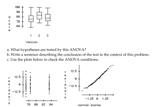
ANOVA table and a boxplot of the results are below.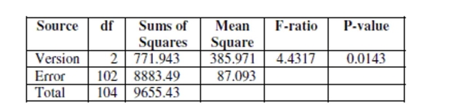
students in her class, she makes 35 copies of each version. The 105 exams are randomly
scrambled, and one copy is given to each student. After the exam, the professor is
concerned that one version might have been easier than the others. She uses a one-way
ANOVA to test whether the average score was different for the three versions. The
ANOVA table and a boxplot of the results are below.
Question
Of the 23 first year male students at State U. admitted from Jim Thorpe High School, 8 were offered baseball scholarships and
7 were offered football scholarships. The University admissions committee looked at the students' composite ACT scores
(shown in the tabl, wondering if the University was lowering their standards for athletes. Assuming that this group of
students is representative of all admitted students, what do you think?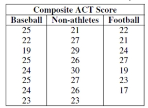
Are the two sports teams mean ACT scores different?
Question
Which of the following are NOT characteristics of a good regression model? 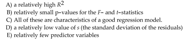
Question
Question
Here are data about the average January low temperature in cities in the United States, and factors that might allow us to
predict temperature. The data, available for 55 cities, include: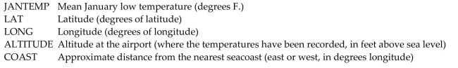 We will attempt to make a regression model to help account for mean January temperature and to understand the effects of
the various predictors.
At each step of the analysis you may assume that things learned earlier in the process are known.
Units Note: The "degrees" of temperature, given here on the Fahrenheit scale, have only coincidental language relationship to
the "degrees" of longitude and latitude. The geographic "degrees" are based on modeling the Earth as a sphere and dividing it
up into 360 degrees for a full circle. Thus 180 degrees of longitude is halfway around the world from Greenwich, England
(0°) and Latitude increases from 0 degrees at the Equator to 90 degrees of (North) latitude at the North Pole.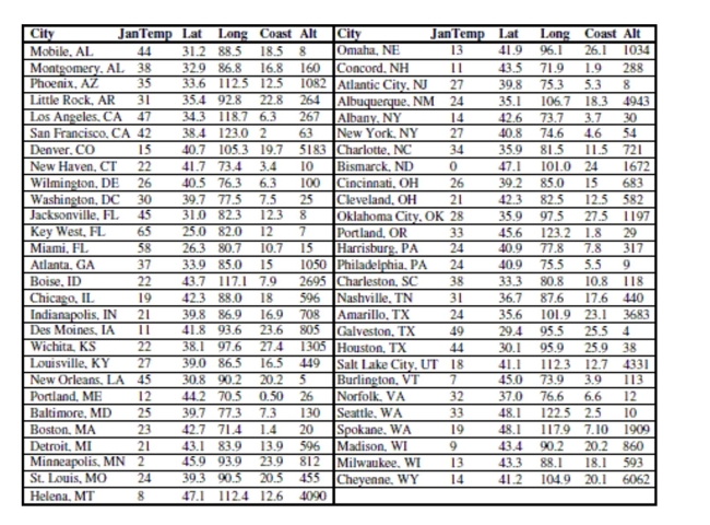
Here is the corresponding regression table: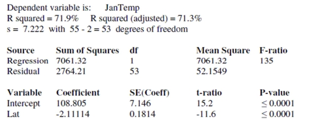
Write a brief report based on this regression. Explain in words and numbers what this
equation says about the relationship between average January low temperature and
latitude. Discuss the R2 value and t-ratios.
predict temperature. The data, available for 55 cities, include:
We will attempt to make a regression model to help account for mean January temperature and to understand the effects ofthe various predictors.
At each step of the analysis you may assume that things learned earlier in the process are known.
Units Note: The "degrees" of temperature, given here on the Fahrenheit scale, have only coincidental language relationship to
the "degrees" of longitude and latitude. The geographic "degrees" are based on modeling the Earth as a sphere and dividing it
up into 360 degrees for a full circle. Thus 180 degrees of longitude is halfway around the world from Greenwich, England
(0°) and Latitude increases from 0 degrees at the Equator to 90 degrees of (North) latitude at the North Pole.
Here is the corresponding regression table:
Write a brief report based on this regression. Explain in words and numbers what this
equation says about the relationship between average January low temperature and
latitude. Discuss the R2 value and t-ratios.
Question
Here are data about the average January low temperature in cities in the United States, and factors that might allow us to
predict temperature. The data, available for 55 cities, include: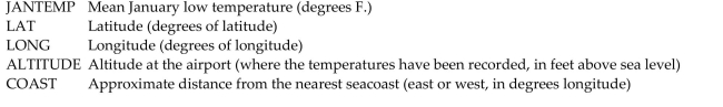 We will attempt to make a regression model to help account for mean January temperature and to understand the effects of
the various predictors.
At each step of the analysis you may assume that things learned earlier in the process are known.
Units Note: The "degrees" of temperature, given here on the Fahrenheit scale, have only coincidental language relationship to
the "degrees" of longitude and latitude. The geographic "degrees" are based on modeling the Earth as a sphere and dividing it
up into 360 degrees for a full circle. Thus 180 degrees of longitude is halfway around the world from Greenwich, England
(0°) and Latitude increases from 0 degrees at the Equator to 90 degrees of (North) latitude at the North Pole.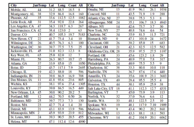
Here is a partial regression plot for the coefficient of Long in the regression with a least
squares regression line added to the display: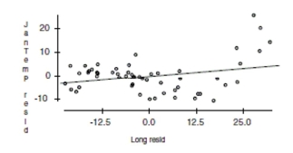
What is the slope of the line on this display? Does the display suggest that this slope
adequately summarizes the effect of longitude in the regression? Why/Why not?
predict temperature. The data, available for 55 cities, include:
We will attempt to make a regression model to help account for mean January temperature and to understand the effects ofthe various predictors.
At each step of the analysis you may assume that things learned earlier in the process are known.
Units Note: The "degrees" of temperature, given here on the Fahrenheit scale, have only coincidental language relationship to
the "degrees" of longitude and latitude. The geographic "degrees" are based on modeling the Earth as a sphere and dividing it
up into 360 degrees for a full circle. Thus 180 degrees of longitude is halfway around the world from Greenwich, England
(0°) and Latitude increases from 0 degrees at the Equator to 90 degrees of (North) latitude at the North Pole.
Here is a partial regression plot for the coefficient of Long in the regression with a least
squares regression line added to the display:
What is the slope of the line on this display? Does the display suggest that this slope
adequately summarizes the effect of longitude in the regression? Why/Why not?
Question
When a sum of squares is divided by its degrees of freedom, the result is called a(n)... 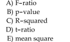
Question
For a class project, students tested four different brands of laundry detergent (1, 2, 3, 4) in
three different water temperatures (hot, warm, cold) to see whether their were any
differences in how well the detergents could clean clothes. The students took 36 identical
pieces of cloth and made them dirty by staining them with coffee, dirt, and grass. The 36
pieces were randomly assigned to the 12 combinations of detergent and temperature so
that each combination had 3 replicates. After washing, the students rated how clean the
clothes were from 0 (no change) to 20 (completely spotless). The two factor ANOVA table
is shown below along with an interaction plot and residual plots.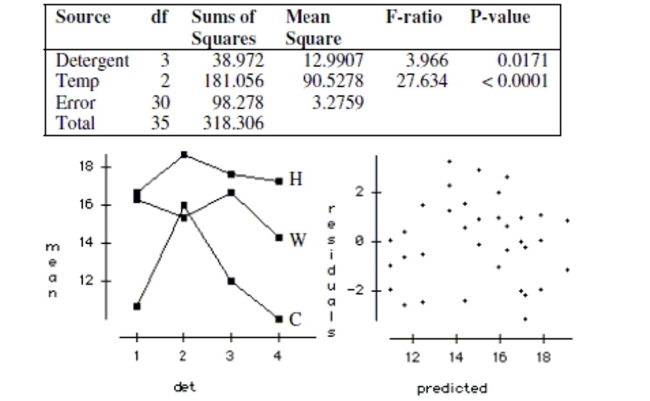
a. Write the hypotheses tested by the Detergent F-ratio. Test the hypotheses and explain
your conclusion in the context of the problem.
b. Write the hypotheses tested by the Temp F-ratio. Test the hypotheses and explain your
conclusion in the context of the problem.
c. Check the conditions required for the ANOVA analysis.
Question
Of the 23 first year male students at State U. admitted from Jim Thorpe High School, 8 were offered baseball scholarships and
7 were offered football scholarships. The University admissions committee looked at the students' composite ACT scores
(shown in the tabl, wondering if the University was lowering their standards for athletes. Assuming that this group of
students is representative of all admitted students, what do you think?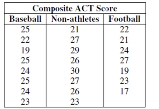
Test an appropriate hypothesis and state your conclusion.
Question
Here are data about the average January low temperature in cities in the United States, and factors that might allow us to
predict temperature. The data, available for 55 cities, include: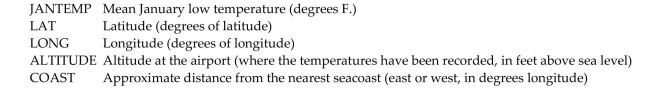 We will attempt to make a regression model to help account for mean January temperature and to understand the effects of
the various predictors.
At each step of the analysis you may assume that things learned earlier in the process are known.
Units Note: The "degrees" of temperature, given here on the Fahrenheit scale, have only coincidental language relationship to
the "degrees" of longitude and latitude. The geographic "degrees" are based on modeling the Earth as a sphere and dividing it
up into 360 degrees for a full circle. Thus 180 degrees of longitude is halfway around the world from Greenwich, England
(0°) and Latitude increases from 0 degrees at the Equator to 90 degrees of (North) latitude at the North Pole.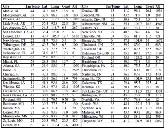
First, we consider the relationship between temperature and latitude. This seems to be the
obvious first choice; everybody knows that northern (high latitude) cities tend to be colder
in January than southern (lower latitude) cities. Here is the scatterplot: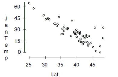
Describe what you see in this scatterplot in a sentence or two. Which of the regression
assumptions for the regression of Jantemp on Lat can you check with this plot? State them
and indicate whether you think they seem to be satisfied.
predict temperature. The data, available for 55 cities, include:
We will attempt to make a regression model to help account for mean January temperature and to understand the effects ofthe various predictors.
At each step of the analysis you may assume that things learned earlier in the process are known.
Units Note: The "degrees" of temperature, given here on the Fahrenheit scale, have only coincidental language relationship to
the "degrees" of longitude and latitude. The geographic "degrees" are based on modeling the Earth as a sphere and dividing it
up into 360 degrees for a full circle. Thus 180 degrees of longitude is halfway around the world from Greenwich, England
(0°) and Latitude increases from 0 degrees at the Equator to 90 degrees of (North) latitude at the North Pole.
First, we consider the relationship between temperature and latitude. This seems to be the
obvious first choice; everybody knows that northern (high latitude) cities tend to be colder
in January than southern (lower latitude) cities. Here is the scatterplot:
Describe what you see in this scatterplot in a sentence or two. Which of the regression
assumptions for the regression of Jantemp on Lat can you check with this plot? State them
and indicate whether you think they seem to be satisfied.
Question
The regression below predicts the daily number of skiers who visit a small ski resort based on three explanatory variables.
The data is a random sample of 30 days from the past two ski seasons. The variables are: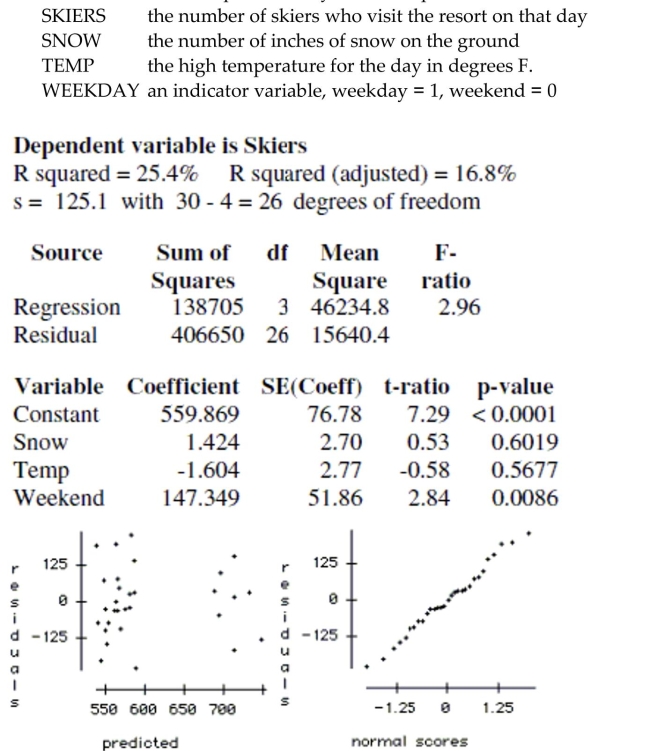
If you think that the temperature might affect attendance differently on weekends than on
weekdays, how would you change the regression to test this?
The data is a random sample of 30 days from the past two ski seasons. The variables are:
If you think that the temperature might affect attendance differently on weekends than on
weekdays, how would you change the regression to test this?
Question
The regression below predicts the daily number of skiers who visit a small ski resort based on three explanatory variables.
The data is a random sample of 30 days from the past two ski seasons. The variables are: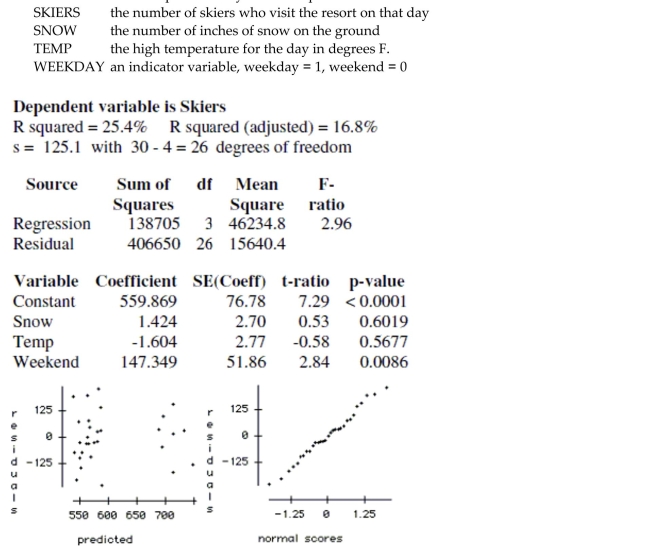
Compute a 95% confidence interval for the slope of the variable Weekend, and explain the
meaning of the interval in the context of the problem.
The data is a random sample of 30 days from the past two ski seasons. The variables are:
Compute a 95% confidence interval for the slope of the variable Weekend, and explain the
meaning of the interval in the context of the problem.
Question
The regression below predicts the daily number of skiers who visit a small ski resort based on three explanatory variables.
The data is a random sample of 30 days from the past two ski seasons. The variables are:
What is the predicted number of skiers for a Saturday with a temperature of 40° F. and a
snow cover of 25 inches?
The data is a random sample of 30 days from the past two ski seasons. The variables are:
What is the predicted number of skiers for a Saturday with a temperature of 40° F. and a
snow cover of 25 inches?
Question
A student wants to build a paper airplane that gets maximum flight distance. She tries
three ways of bending the wing (down, flat, and up) and two levels of nose weight (no and yes
- a paper clip). She randomizes the 12 runs (each condition replicated twice). The analysis
of variance for the 12 runs is shown in the table below along with an interaction plot and
tables of the mean distance for the different wing bends and weights.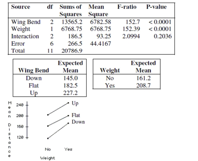
a. Does an additive model seem adequate? Explain.
b. Write a report on this analysis of the data. Include any recommendations you would
give the student on designing the plane.
Question
Here are data about the average January low temperature in cities in the United States, and factors that might allow us to
predict temperature. The data, available for 55 cities, include: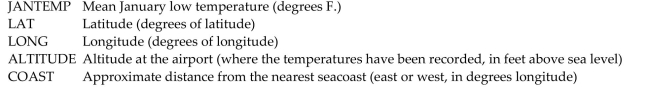 We will attempt to make a regression model to help account for mean January temperature and to understand the effects of
the various predictors.
At each step of the analysis you may assume that things learned earlier in the process are known.
Units Note: The "degrees" of temperature, given here on the Fahrenheit scale, have only coincidental language relationship to
the "degrees" of longitude and latitude. The geographic "degrees" are based on modeling the Earth as a sphere and dividing it
up into 360 degrees for a full circle. Thus 180 degrees of longitude is halfway around the world from Greenwich, England
(0°) and Latitude increases from 0 degrees at the Equator to 90 degrees of (North) latitude at the North Pole.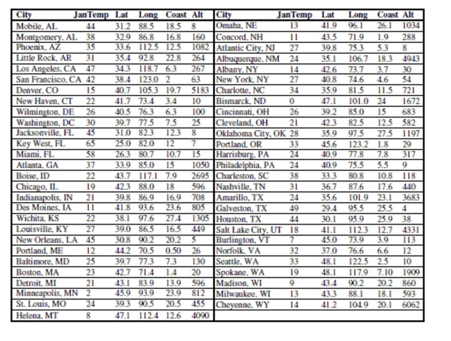
Here is the regression with both Latitude and Longitude as predictors: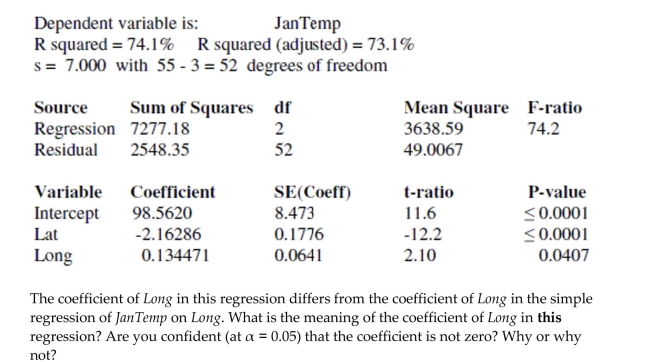
predict temperature. The data, available for 55 cities, include:
We will attempt to make a regression model to help account for mean January temperature and to understand the effects ofthe various predictors.
At each step of the analysis you may assume that things learned earlier in the process are known.
Units Note: The "degrees" of temperature, given here on the Fahrenheit scale, have only coincidental language relationship to
the "degrees" of longitude and latitude. The geographic "degrees" are based on modeling the Earth as a sphere and dividing it
up into 360 degrees for a full circle. Thus 180 degrees of longitude is halfway around the world from Greenwich, England
(0°) and Latitude increases from 0 degrees at the Equator to 90 degrees of (North) latitude at the North Pole.
Here is the regression with both Latitude and Longitude as predictors:
Question
Here are data about the average January low temperature in cities in the United States, and factors that might allow us to
predict temperature. The data, available for 55 cities, include: We will attempt to make a regression model to help account for mean January temperature and to understand the effects of
the various predictors.
At each step of the analysis you may assume that things learned earlier in the process are known.
Units Note: The "degrees" of temperature, given here on the Fahrenheit scale, have only coincidental language relationship to
the "degrees" of longitude and latitude. The geographic "degrees" are based on modeling the Earth as a sphere and dividing it
up into 360 degrees for a full circle. Thus 180 degrees of longitude is halfway around the world from Greenwich, England
(0°) and Latitude increases from 0 degrees at the Equator to 90 degrees of (North) latitude at the North Pole.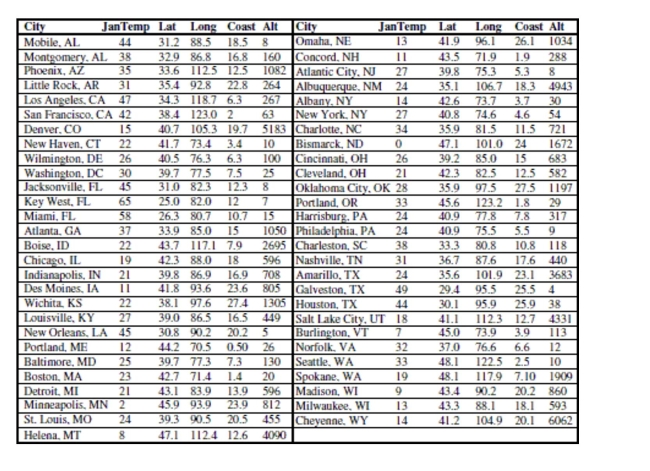
Now, consider longitude. Should the longitude of a city have an influence on average
January low temperature? Here is the regression: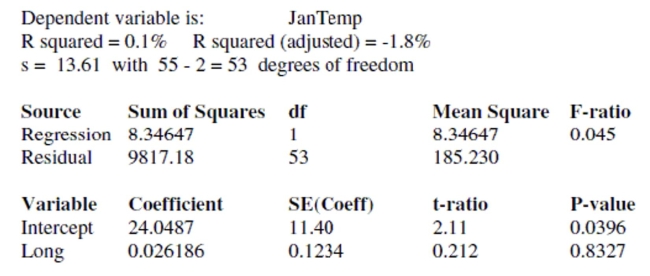
Test the null hypothesis that the true coefficient of Long is zero in this regression. State the
null and alternative hypotheses and indicate your procedure and conclusion.
predict temperature. The data, available for 55 cities, include:
We will attempt to make a regression model to help account for mean January temperature and to understand the effects ofthe various predictors.
At each step of the analysis you may assume that things learned earlier in the process are known.
Units Note: The "degrees" of temperature, given here on the Fahrenheit scale, have only coincidental language relationship to
the "degrees" of longitude and latitude. The geographic "degrees" are based on modeling the Earth as a sphere and dividing it
up into 360 degrees for a full circle. Thus 180 degrees of longitude is halfway around the world from Greenwich, England
(0°) and Latitude increases from 0 degrees at the Equator to 90 degrees of (North) latitude at the North Pole.
Now, consider longitude. Should the longitude of a city have an influence on average
January low temperature? Here is the regression:
Test the null hypothesis that the true coefficient of Long is zero in this regression. State the
null and alternative hypotheses and indicate your procedure and conclusion.
Question
Three brands of AAA batteries are compared to see which last longest. Each brand of
battery is tested in four different devices (a TV remote control, a hand-held game, a
miniature flashlight, and a digital camera). The experiment is run once for each
combination of brand and device. The twelve runs are ordered randomly. The time that the
each battery lasts (in minutes) under continuous usage is recorded.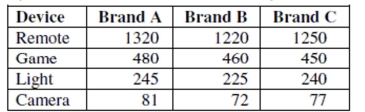
The two-way ANOVA table for response variable Time and factors Brand and Device is
given below.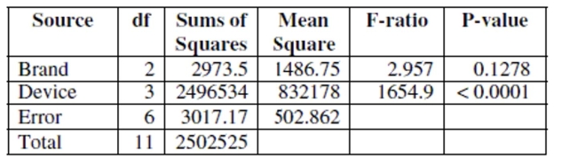
a. Write the model equation for this ANOVA. (Use symbols or words, no numbers.)
b. Test to see whether there is a brand effect. Write the hypotheses being tested, and state
your conclusion using a 5% level of significance. Write your conclusion in the context of
this problem.
c. Explain the role that the device factor plays in this analysis.
d. Can an interaction term be added to this model? Explain.
e. Use the plots below to check the ANOVA conditions.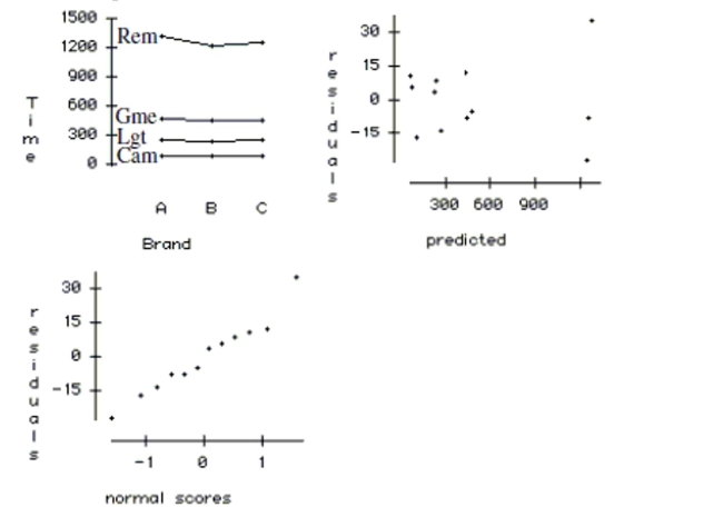
Question
The regression below predicts the daily number of skiers who visit a small ski resort based on three explanatory variables.
The data is a random sample of 30 days from the past two ski seasons. The variables are: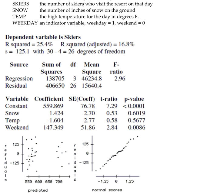
Which of the explanatory variables appear to be associated with the number of skiers, and
which do not? Explain how you reached your conclusion.
The data is a random sample of 30 days from the past two ski seasons. The variables are:
Which of the explanatory variables appear to be associated with the number of skiers, and
which do not? Explain how you reached your conclusion.

Unlock Deck
Sign up to unlock the cards in this deck!
Unlock Deck
Unlock Deck
1/25
Play
Full screen (f)
Deck 7: Inference When Variables Are Related
1
In ANOVA, an interaction between two factors means that…
A) the effect of one factor depends on the level of the other factor.
B) the variances of the two factors are unequal.
C) none of these
D) both factors are related to the response variable.
E) the data was not collected using randomization.
A) the effect of one factor depends on the level of the other factor.
B) the variances of the two factors are unequal.
C) none of these
D) both factors are related to the response variable.
E) the data was not collected using randomization.
A
2
Homelessness is a problem in many large U.S. cities. To better understand the problem, a
multiple regression was used to model the rate of homelessness based on several
explanatory variables. The following data were collected for 50 large U.S. cities. The
regression results appear below.
a. Using a 5% level of significance, which variables are associated with the number of
homeless in a city?
b. Explain the meaning of the coefficient of temperature in the context of this problem.
c. Explain the meaning of the coefficient of rent control in the context of this problem.
d. Do the results suggest that having rent control laws in a city causes higher levels of
homelessness? Explain.
e. If we created a new model by adding several more explanatory variables, which statistic
should be used to compare them - the R2 or the adjusted R2 ? Explain.
f. Using the plots below, check the regression conditions.
no obvious curvature. (We should also check plots of Homeless vs. each X variable.)
* Does the plot thicken? condition: OK. The plot of residuals vs. predicted values is
approximately the same width throughout.
* Randomization condition: Caution. We do not know whether or not the 50 U.S.
cities in our sample were chosen randomly, or whether they are representative of all
large U.S. cities.
* Nearly Normal condition: Violated. The normal probability plot is curved, which
indicates that the regression errors do not follow a Normal model. (It may be
possible to re-express the y-variable to fix this problem.)
3
In regression an observation has high leverage when
A) none of these
B) the observation is poorly predicted by the regression.
C) the observation has a combination of x-values that is far from the center of the data.
D) removing the observation causes a large change in one of more coefficients of the model.
E) the observation is perfectly predicted by the regression.
C
4
Check the conditions for the regression and comment on whether or not they are satisfied.
Unlock Deck
Unlock for access to all 25 flashcards in this deck.
Unlock Deck
k this deck
5
Engineers want to know what factors are associated with gas mileage. The regression
below predicts the average miles per gallon (MPG) for 82 cars using their engine
horsepower (HP) and weight (WT, in 100's of pounds).
a. Write down the regression equation.
b. Write down the hypotheses for the test of the coefficient of horsepower. Conduct the test
and explain your conclusion in the context of this problem.
c. Write down the hypotheses for the test of the coefficient of weight. Conduct the test and
explain your conclusion in the context of this problem.
d. Explain the meaning of the coefficient of weight in the context of this problem.
e. Explain the meaning of the intercept of this regression in the context of this problem.
f. Compute the predicted gas mileage of a 3500 pound car with a 150 horsepower engine.
The plots are MPG vs. HP, MPG vs. WT, residuals vs. predicted values, and a normal
probability plot of residuals.
g. Check the conditions of this regression and comment on whether they are satisfied.
Unlock Deck
Unlock for access to all 25 flashcards in this deck.
Unlock Deck
k this deck
6
Here are data about the average January low temperature in cities in the United States, and factors that might allow us to
predict temperature. The data, available for 55 cities, include: We will attempt to make a regression model to help account for mean January temperature and to understand the effects of
the various predictors.
At each step of the analysis you may assume that things learned earlier in the process are known.
Units Note: The "degrees" of temperature, given here on the Fahrenheit scale, have only coincidental language relationship to
the "degrees" of longitude and latitude. The geographic "degrees" are based on modeling the Earth as a sphere and dividing it
up into 360 degrees for a full circle. Thus 180 degrees of longitude is halfway around the world from Greenwich, England
(0°) and Latitude increases from 0 degrees at the Equator to 90 degrees of (North) latitude at the North Pole.
It is possible that the distance that a city is from the ocean could affect its average January
low temperature. Coast gives an approximate distance of each city from the East Coast or
West Coast (whichever is nearer). Including it in the regression yields the following
regression table:
And here is a scatterplot of the residuals:
predict temperature. The data, available for 55 cities, include:
We will attempt to make a regression model to help account for mean January temperature and to understand the effects ofthe various predictors.
At each step of the analysis you may assume that things learned earlier in the process are known.
Units Note: The "degrees" of temperature, given here on the Fahrenheit scale, have only coincidental language relationship to
the "degrees" of longitude and latitude. The geographic "degrees" are based on modeling the Earth as a sphere and dividing it
up into 360 degrees for a full circle. Thus 180 degrees of longitude is halfway around the world from Greenwich, England
(0°) and Latitude increases from 0 degrees at the Equator to 90 degrees of (North) latitude at the North Pole.
It is possible that the distance that a city is from the ocean could affect its average January
low temperature. Coast gives an approximate distance of each city from the East Coast or
West Coast (whichever is nearer). Including it in the regression yields the following
regression table:
And here is a scatterplot of the residuals:
Unlock Deck
Unlock for access to all 25 flashcards in this deck.
Unlock Deck
k this deck
7
In ANOVA, the Bonferroni method is used to...
A) adjust for multiple comparisons between pairs of treatment groups.
B) none of these
C) adjust for unequal variances between the treatment groups.
D) adjust for non-Normal data within the treatment groups.
E) adjust for small sample sizes within the treatment groups.
A) adjust for multiple comparisons between pairs of treatment groups.
B) none of these
C) adjust for unequal variances between the treatment groups.
D) adjust for non-Normal data within the treatment groups.
E) adjust for small sample sizes within the treatment groups.
Unlock Deck
Unlock for access to all 25 flashcards in this deck.
Unlock Deck
k this deck
8
To discourage cheating, a professor makes three different versions of an exam. For the 105
students in her class, she makes 35 copies of each version. The 105 exams are randomly
scrambled, and one copy is given to each student. After the exam, the professor is
concerned that one version might have been easier than the others. She uses a one-way
ANOVA to test whether the average score was different for the three versions. The
ANOVA table and a boxplot of the results are below.
Unlock Deck
Unlock for access to all 25 flashcards in this deck.
Unlock Deck
k this deck
9
Of the 23 first year male students at State U. admitted from Jim Thorpe High School, 8 were offered baseball scholarships and
7 were offered football scholarships. The University admissions committee looked at the students' composite ACT scores
(shown in the tabl, wondering if the University was lowering their standards for athletes. Assuming that this group of
students is representative of all admitted students, what do you think?
Are the two sports teams mean ACT scores different?
Unlock Deck
Unlock for access to all 25 flashcards in this deck.
Unlock Deck
k this deck
10
Which of the following are NOT characteristics of a good regression model?
Unlock Deck
Unlock for access to all 25 flashcards in this deck.
Unlock Deck
k this deck
11
The problem of collinearity occurs when
A) at least one predictor var. has a nonlinear relationship with the response variable.
B) there is an influential observation in the data set.
C) none of these
D) more than one predictor variable is linearly related to the response variable.
E) two or more predictor variables are linearly related to each other.
Unlock Deck
Unlock for access to all 25 flashcards in this deck.
Unlock Deck
k this deck
12
Here are data about the average January low temperature in cities in the United States, and factors that might allow us to
predict temperature. The data, available for 55 cities, include: We will attempt to make a regression model to help account for mean January temperature and to understand the effects of
the various predictors.
At each step of the analysis you may assume that things learned earlier in the process are known.
Units Note: The "degrees" of temperature, given here on the Fahrenheit scale, have only coincidental language relationship to
the "degrees" of longitude and latitude. The geographic "degrees" are based on modeling the Earth as a sphere and dividing it
up into 360 degrees for a full circle. Thus 180 degrees of longitude is halfway around the world from Greenwich, England
(0°) and Latitude increases from 0 degrees at the Equator to 90 degrees of (North) latitude at the North Pole.
Here is the corresponding regression table:
Write a brief report based on this regression. Explain in words and numbers what this
equation says about the relationship between average January low temperature and
latitude. Discuss the R2 value and t-ratios.
predict temperature. The data, available for 55 cities, include:
We will attempt to make a regression model to help account for mean January temperature and to understand the effects ofthe various predictors.
At each step of the analysis you may assume that things learned earlier in the process are known.
Units Note: The "degrees" of temperature, given here on the Fahrenheit scale, have only coincidental language relationship to
the "degrees" of longitude and latitude. The geographic "degrees" are based on modeling the Earth as a sphere and dividing it
up into 360 degrees for a full circle. Thus 180 degrees of longitude is halfway around the world from Greenwich, England
(0°) and Latitude increases from 0 degrees at the Equator to 90 degrees of (North) latitude at the North Pole.
Here is the corresponding regression table:
Write a brief report based on this regression. Explain in words and numbers what this
equation says about the relationship between average January low temperature and
latitude. Discuss the R2 value and t-ratios.
Unlock Deck
Unlock for access to all 25 flashcards in this deck.
Unlock Deck
k this deck
13
Here are data about the average January low temperature in cities in the United States, and factors that might allow us to
predict temperature. The data, available for 55 cities, include: We will attempt to make a regression model to help account for mean January temperature and to understand the effects of
the various predictors.
At each step of the analysis you may assume that things learned earlier in the process are known.
Units Note: The "degrees" of temperature, given here on the Fahrenheit scale, have only coincidental language relationship to
the "degrees" of longitude and latitude. The geographic "degrees" are based on modeling the Earth as a sphere and dividing it
up into 360 degrees for a full circle. Thus 180 degrees of longitude is halfway around the world from Greenwich, England
(0°) and Latitude increases from 0 degrees at the Equator to 90 degrees of (North) latitude at the North Pole.
Here is a partial regression plot for the coefficient of Long in the regression with a least
squares regression line added to the display:
What is the slope of the line on this display? Does the display suggest that this slope
adequately summarizes the effect of longitude in the regression? Why/Why not?
predict temperature. The data, available for 55 cities, include:
We will attempt to make a regression model to help account for mean January temperature and to understand the effects ofthe various predictors.
At each step of the analysis you may assume that things learned earlier in the process are known.
Units Note: The "degrees" of temperature, given here on the Fahrenheit scale, have only coincidental language relationship to
the "degrees" of longitude and latitude. The geographic "degrees" are based on modeling the Earth as a sphere and dividing it
up into 360 degrees for a full circle. Thus 180 degrees of longitude is halfway around the world from Greenwich, England
(0°) and Latitude increases from 0 degrees at the Equator to 90 degrees of (North) latitude at the North Pole.
Here is a partial regression plot for the coefficient of Long in the regression with a least
squares regression line added to the display:
What is the slope of the line on this display? Does the display suggest that this slope
adequately summarizes the effect of longitude in the regression? Why/Why not?
Unlock Deck
Unlock for access to all 25 flashcards in this deck.
Unlock Deck
k this deck
14
When a sum of squares is divided by its degrees of freedom, the result is called a(n)...
Unlock Deck
Unlock for access to all 25 flashcards in this deck.
Unlock Deck
k this deck
15
For a class project, students tested four different brands of laundry detergent (1, 2, 3, 4) in
three different water temperatures (hot, warm, cold) to see whether their were any
differences in how well the detergents could clean clothes. The students took 36 identical
pieces of cloth and made them dirty by staining them with coffee, dirt, and grass. The 36
pieces were randomly assigned to the 12 combinations of detergent and temperature so
that each combination had 3 replicates. After washing, the students rated how clean the
clothes were from 0 (no change) to 20 (completely spotless). The two factor ANOVA table
is shown below along with an interaction plot and residual plots.
a. Write the hypotheses tested by the Detergent F-ratio. Test the hypotheses and explain
your conclusion in the context of the problem.
b. Write the hypotheses tested by the Temp F-ratio. Test the hypotheses and explain your
conclusion in the context of the problem.
c. Check the conditions required for the ANOVA analysis.
three different water temperatures (hot, warm, cold) to see whether their were any
differences in how well the detergents could clean clothes. The students took 36 identical
pieces of cloth and made them dirty by staining them with coffee, dirt, and grass. The 36
pieces were randomly assigned to the 12 combinations of detergent and temperature so
that each combination had 3 replicates. After washing, the students rated how clean the
clothes were from 0 (no change) to 20 (completely spotless). The two factor ANOVA table
is shown below along with an interaction plot and residual plots.
a. Write the hypotheses tested by the Detergent F-ratio. Test the hypotheses and explain
your conclusion in the context of the problem.
b. Write the hypotheses tested by the Temp F-ratio. Test the hypotheses and explain your
conclusion in the context of the problem.
c. Check the conditions required for the ANOVA analysis.
Unlock Deck
Unlock for access to all 25 flashcards in this deck.
Unlock Deck
k this deck
16
Of the 23 first year male students at State U. admitted from Jim Thorpe High School, 8 were offered baseball scholarships and
7 were offered football scholarships. The University admissions committee looked at the students' composite ACT scores
(shown in the tabl, wondering if the University was lowering their standards for athletes. Assuming that this group of
students is representative of all admitted students, what do you think?
Test an appropriate hypothesis and state your conclusion.
Unlock Deck
Unlock for access to all 25 flashcards in this deck.
Unlock Deck
k this deck
17
Here are data about the average January low temperature in cities in the United States, and factors that might allow us to
predict temperature. The data, available for 55 cities, include: We will attempt to make a regression model to help account for mean January temperature and to understand the effects of
the various predictors.
At each step of the analysis you may assume that things learned earlier in the process are known.
Units Note: The "degrees" of temperature, given here on the Fahrenheit scale, have only coincidental language relationship to
the "degrees" of longitude and latitude. The geographic "degrees" are based on modeling the Earth as a sphere and dividing it
up into 360 degrees for a full circle. Thus 180 degrees of longitude is halfway around the world from Greenwich, England
(0°) and Latitude increases from 0 degrees at the Equator to 90 degrees of (North) latitude at the North Pole.
First, we consider the relationship between temperature and latitude. This seems to be the
obvious first choice; everybody knows that northern (high latitude) cities tend to be colder
in January than southern (lower latitude) cities. Here is the scatterplot:
Describe what you see in this scatterplot in a sentence or two. Which of the regression
assumptions for the regression of Jantemp on Lat can you check with this plot? State them
and indicate whether you think they seem to be satisfied.
predict temperature. The data, available for 55 cities, include:
We will attempt to make a regression model to help account for mean January temperature and to understand the effects ofthe various predictors.
At each step of the analysis you may assume that things learned earlier in the process are known.
Units Note: The "degrees" of temperature, given here on the Fahrenheit scale, have only coincidental language relationship to
the "degrees" of longitude and latitude. The geographic "degrees" are based on modeling the Earth as a sphere and dividing it
up into 360 degrees for a full circle. Thus 180 degrees of longitude is halfway around the world from Greenwich, England
(0°) and Latitude increases from 0 degrees at the Equator to 90 degrees of (North) latitude at the North Pole.
First, we consider the relationship between temperature and latitude. This seems to be the
obvious first choice; everybody knows that northern (high latitude) cities tend to be colder
in January than southern (lower latitude) cities. Here is the scatterplot:
Describe what you see in this scatterplot in a sentence or two. Which of the regression
assumptions for the regression of Jantemp on Lat can you check with this plot? State them
and indicate whether you think they seem to be satisfied.
Unlock Deck
Unlock for access to all 25 flashcards in this deck.
Unlock Deck
k this deck
18
The regression below predicts the daily number of skiers who visit a small ski resort based on three explanatory variables.
The data is a random sample of 30 days from the past two ski seasons. The variables are:
If you think that the temperature might affect attendance differently on weekends than on
weekdays, how would you change the regression to test this?
The data is a random sample of 30 days from the past two ski seasons. The variables are:
If you think that the temperature might affect attendance differently on weekends than on
weekdays, how would you change the regression to test this?
Unlock Deck
Unlock for access to all 25 flashcards in this deck.
Unlock Deck
k this deck
19
The regression below predicts the daily number of skiers who visit a small ski resort based on three explanatory variables.
The data is a random sample of 30 days from the past two ski seasons. The variables are:
Compute a 95% confidence interval for the slope of the variable Weekend, and explain the
meaning of the interval in the context of the problem.
The data is a random sample of 30 days from the past two ski seasons. The variables are:
Compute a 95% confidence interval for the slope of the variable Weekend, and explain the
meaning of the interval in the context of the problem.
Unlock Deck
Unlock for access to all 25 flashcards in this deck.
Unlock Deck
k this deck
20
The regression below predicts the daily number of skiers who visit a small ski resort based on three explanatory variables.
The data is a random sample of 30 days from the past two ski seasons. The variables are:
What is the predicted number of skiers for a Saturday with a temperature of 40° F. and a
snow cover of 25 inches?
The data is a random sample of 30 days from the past two ski seasons. The variables are:
What is the predicted number of skiers for a Saturday with a temperature of 40° F. and a
snow cover of 25 inches?
Unlock Deck
Unlock for access to all 25 flashcards in this deck.
Unlock Deck
k this deck
21
A student wants to build a paper airplane that gets maximum flight distance. She tries
three ways of bending the wing (down, flat, and up) and two levels of nose weight (no and yes
- a paper clip). She randomizes the 12 runs (each condition replicated twice). The analysis
of variance for the 12 runs is shown in the table below along with an interaction plot and
tables of the mean distance for the different wing bends and weights.
a. Does an additive model seem adequate? Explain.
b. Write a report on this analysis of the data. Include any recommendations you would
give the student on designing the plane.
three ways of bending the wing (down, flat, and up) and two levels of nose weight (no and yes
- a paper clip). She randomizes the 12 runs (each condition replicated twice). The analysis
of variance for the 12 runs is shown in the table below along with an interaction plot and
tables of the mean distance for the different wing bends and weights.
a. Does an additive model seem adequate? Explain.
b. Write a report on this analysis of the data. Include any recommendations you would
give the student on designing the plane.
Unlock Deck
Unlock for access to all 25 flashcards in this deck.
Unlock Deck
k this deck
22
Here are data about the average January low temperature in cities in the United States, and factors that might allow us to
predict temperature. The data, available for 55 cities, include: We will attempt to make a regression model to help account for mean January temperature and to understand the effects of
the various predictors.
At each step of the analysis you may assume that things learned earlier in the process are known.
Units Note: The "degrees" of temperature, given here on the Fahrenheit scale, have only coincidental language relationship to
the "degrees" of longitude and latitude. The geographic "degrees" are based on modeling the Earth as a sphere and dividing it
up into 360 degrees for a full circle. Thus 180 degrees of longitude is halfway around the world from Greenwich, England
(0°) and Latitude increases from 0 degrees at the Equator to 90 degrees of (North) latitude at the North Pole.
Here is the regression with both Latitude and Longitude as predictors:
predict temperature. The data, available for 55 cities, include:
We will attempt to make a regression model to help account for mean January temperature and to understand the effects ofthe various predictors.
At each step of the analysis you may assume that things learned earlier in the process are known.
Units Note: The "degrees" of temperature, given here on the Fahrenheit scale, have only coincidental language relationship to
the "degrees" of longitude and latitude. The geographic "degrees" are based on modeling the Earth as a sphere and dividing it
up into 360 degrees for a full circle. Thus 180 degrees of longitude is halfway around the world from Greenwich, England
(0°) and Latitude increases from 0 degrees at the Equator to 90 degrees of (North) latitude at the North Pole.
Here is the regression with both Latitude and Longitude as predictors:
Unlock Deck
Unlock for access to all 25 flashcards in this deck.
Unlock Deck
k this deck
23
Here are data about the average January low temperature in cities in the United States, and factors that might allow us to
predict temperature. The data, available for 55 cities, include: We will attempt to make a regression model to help account for mean January temperature and to understand the effects of
the various predictors.
At each step of the analysis you may assume that things learned earlier in the process are known.
Units Note: The "degrees" of temperature, given here on the Fahrenheit scale, have only coincidental language relationship to
the "degrees" of longitude and latitude. The geographic "degrees" are based on modeling the Earth as a sphere and dividing it
up into 360 degrees for a full circle. Thus 180 degrees of longitude is halfway around the world from Greenwich, England
(0°) and Latitude increases from 0 degrees at the Equator to 90 degrees of (North) latitude at the North Pole.
Now, consider longitude. Should the longitude of a city have an influence on average
January low temperature? Here is the regression:
Test the null hypothesis that the true coefficient of Long is zero in this regression. State the
null and alternative hypotheses and indicate your procedure and conclusion.
predict temperature. The data, available for 55 cities, include:
We will attempt to make a regression model to help account for mean January temperature and to understand the effects ofthe various predictors.
At each step of the analysis you may assume that things learned earlier in the process are known.
Units Note: The "degrees" of temperature, given here on the Fahrenheit scale, have only coincidental language relationship to
the "degrees" of longitude and latitude. The geographic "degrees" are based on modeling the Earth as a sphere and dividing it
up into 360 degrees for a full circle. Thus 180 degrees of longitude is halfway around the world from Greenwich, England
(0°) and Latitude increases from 0 degrees at the Equator to 90 degrees of (North) latitude at the North Pole.
Now, consider longitude. Should the longitude of a city have an influence on average
January low temperature? Here is the regression:
Test the null hypothesis that the true coefficient of Long is zero in this regression. State the
null and alternative hypotheses and indicate your procedure and conclusion.
Unlock Deck
Unlock for access to all 25 flashcards in this deck.
Unlock Deck
k this deck
24
Three brands of AAA batteries are compared to see which last longest. Each brand of
battery is tested in four different devices (a TV remote control, a hand-held game, a
miniature flashlight, and a digital camera). The experiment is run once for each
combination of brand and device. The twelve runs are ordered randomly. The time that the
each battery lasts (in minutes) under continuous usage is recorded.
The two-way ANOVA table for response variable Time and factors Brand and Device is
given below.
a. Write the model equation for this ANOVA. (Use symbols or words, no numbers.)
b. Test to see whether there is a brand effect. Write the hypotheses being tested, and state
your conclusion using a 5% level of significance. Write your conclusion in the context of
this problem.
c. Explain the role that the device factor plays in this analysis.
d. Can an interaction term be added to this model? Explain.
e. Use the plots below to check the ANOVA conditions.
battery is tested in four different devices (a TV remote control, a hand-held game, a
miniature flashlight, and a digital camera). The experiment is run once for each
combination of brand and device. The twelve runs are ordered randomly. The time that the
each battery lasts (in minutes) under continuous usage is recorded.
The two-way ANOVA table for response variable Time and factors Brand and Device is
given below.
a. Write the model equation for this ANOVA. (Use symbols or words, no numbers.)
b. Test to see whether there is a brand effect. Write the hypotheses being tested, and state
your conclusion using a 5% level of significance. Write your conclusion in the context of
this problem.
c. Explain the role that the device factor plays in this analysis.
d. Can an interaction term be added to this model? Explain.
e. Use the plots below to check the ANOVA conditions.
Unlock Deck
Unlock for access to all 25 flashcards in this deck.
Unlock Deck
k this deck
25
The regression below predicts the daily number of skiers who visit a small ski resort based on three explanatory variables.
The data is a random sample of 30 days from the past two ski seasons. The variables are:
Which of the explanatory variables appear to be associated with the number of skiers, and
which do not? Explain how you reached your conclusion.
The data is a random sample of 30 days from the past two ski seasons. The variables are:
Which of the explanatory variables appear to be associated with the number of skiers, and
which do not? Explain how you reached your conclusion.
Unlock Deck
Unlock for access to all 25 flashcards in this deck.
Unlock Deck
k this deck
Unlock Deck
Unlock for access to all 25 flashcards in this deck.


