Deck 11: Simple Linear Regression
Full screen (f)
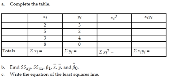
Question
Is the number of games won by a major league baseball team in a season related to the team's batting average? Data from 14 teams were collected and the summary statistics yield:  Find the least squares prediction equation for predicting the number of games won, y, using a straight-line relationship with the team's batting average, x.
Find the least squares prediction equation for predicting the number of games won, y, using a straight-line relationship with the team's batting average, x. Question
To investigate the relationship between yield of potatoes, y, and level of fertilizer application, x, a researcher divides a field into eight plots of equal size and applies differing amounts of fertilizer to each. The yield of potatoes (in pounds) and the fertilizer application (in pounds) are recorded for each plot. The data are as follows: 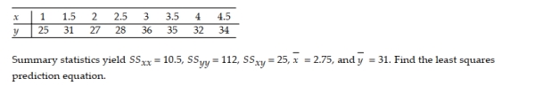
Question
(0, 6) and (6, 0) 

Question

Question
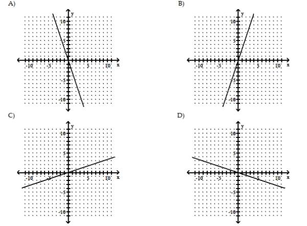
(-6, 0) and (-3, -1) 
Question
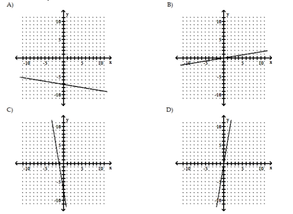
(2, -6) and (-1, 3) 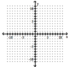
Question
Question
(-7, -6) and (-1, -7) 
Question
Question
Question
(-8, -8) and (4, 4) 
Question
Question
Consider the following pairs of measurements: 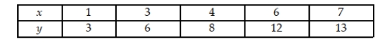 a. Construct a scattergram for the data. b. What does the scattergram suggest about the relationship between x and y? c. Find the least squares estimates of β0 and β1. d. Plot the least squares line on your scattergram. Does the line appear to fit the data well?
a. Construct a scattergram for the data. b. What does the scattergram suggest about the relationship between x and y? c. Find the least squares estimates of β0 and β1. d. Plot the least squares line on your scattergram. Does the line appear to fit the data well? Question
In a study of feeding behavior, zoologists recorded the number of grunts of a warthog feeding by a lake in the 15 minute period following the addition of food. The data showing the number of grunts and and the age of the warthog (in days) are listed below: 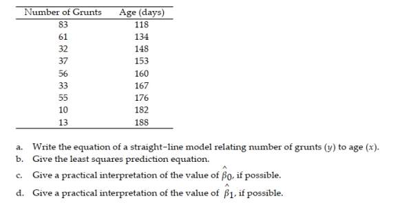
Question
A county real estate appraiser wants to develop a statistical model to predict the appraised value of houses in a section of the county called East Meadow. One of the many variables thought to be an important predictor of appraised value is the number of rooms in the house. Consequently, the appraiser decided to fit the simple linear regression model: 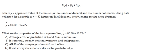
Question
In a comprehensive road test for new car models, one variable measured is the time it takes the car to accelerate from 0 to 60 miles per hour. To model acceleration time, a regression analysis is conducted on a random sample of 129 new cars. TIME60: y = Elapsed time (in seconds) from 0 mph to 60 mph MAX: x = Maximum speed attained (miles per hour) 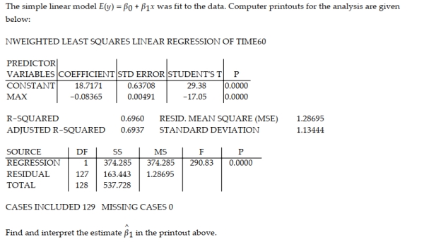
Question
Question
Question
Is there a relationship between the raises administrators at County University receive and their performance on the job? A faculty group wants to determine whether job rating (x) is a useful linear predictor of raise (y). Consequently, the group considered the linear regression model 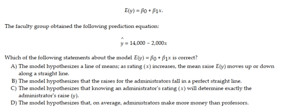
Question
Question
Suppose you fit a least squares line to 25 data points and the calculated value of SSE is 0.42. 
Question
What is the relationship between diamond price and carat size? 307 diamonds were sampled and a straight-line relationship was hypothesized between y = diamond price (in dollars) and x = size of the diamond (in carats). The simple linear regression for the analysis is shown below: Least Squares Linear Regression of PRICE 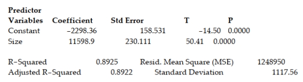 Which of the following assumptions is not stated correctly?
A) The probability distribution of ε is normal.
B) The mean of the probability distribution of ε is 0.
C) The variance of the probability distribution of ε is constant for all settings of the independent variable.
D) The values of ε associated with any two observations are dependent on one another.
Which of the following assumptions is not stated correctly?A) The probability distribution of ε is normal.
B) The mean of the probability distribution of ε is 0.
C) The variance of the probability distribution of ε is constant for all settings of the independent variable.
D) The values of ε associated with any two observations are dependent on one another.
Question
Question
Question
Question
Question
Question
What is the relationship between diamond price and carat size? 307 diamonds were sampled (ranging in size from 0.18 to 1.1 carats) and a straight-line relationship was hypothesized between y = diamond price (in dollars) and x = size of the diamond (in carats). The simple linear regression for the analysis is shown below: Least Squares Linear Regression of PRICE 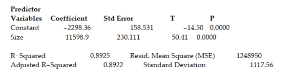 Interpret the estimated y-intercept of the regression line.
A) When a diamond is 0 carats in size, we estimate the price of the diamond to be $11,598.90.
B) When a diamond is 0 carats in size, we estimate the price of the diamond to be $2298.36.
C) When a diamond is 11598.9 carats in size, we estimate the price of the diamond to be $2298.36.
D) No practical interpretation of the y-intercept exists since a diamond of 0 carats cannot exist and falls outside the range of the carat sizes sampled.
Interpret the estimated y-intercept of the regression line.A) When a diamond is 0 carats in size, we estimate the price of the diamond to be $11,598.90.
B) When a diamond is 0 carats in size, we estimate the price of the diamond to be $2298.36.
C) When a diamond is 11598.9 carats in size, we estimate the price of the diamond to be $2298.36.
D) No practical interpretation of the y-intercept exists since a diamond of 0 carats cannot exist and falls outside the range of the carat sizes sampled.
Question

Question
Question
What is the relationship between diamond price and carat size? 307 diamonds were sampled and a straight-line relationship was hypothesized between y = diamond price (in dollars) and x = size of the diamond (in carats). The simple linear regression for the analysis is shown below: Least Squares Linear Regression of PRICE 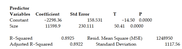 Interpret the standard deviation of the regression model.
A) We can explain 89.25% of the variation in the sampled diamond prices around their mean using the size of the diamond in a linear model.
B) We expect most of the sampled diamond prices to fall within $1117.56 of their least squares predicted values.
C) We expect most of the sampled diamond prices to fall within $2235.12 of their least squares predicted values.
D) For every 1-carat increase in the size of a diamond, we estimate that the price of the diamond will increase by $1117.56.
Interpret the standard deviation of the regression model.A) We can explain 89.25% of the variation in the sampled diamond prices around their mean using the size of the diamond in a linear model.
B) We expect most of the sampled diamond prices to fall within $1117.56 of their least squares predicted values.
C) We expect most of the sampled diamond prices to fall within $2235.12 of their least squares predicted values.
D) For every 1-carat increase in the size of a diamond, we estimate that the price of the diamond will increase by $1117.56.
Question
Question

Question
Question
What is the relationship between diamond price and carat size? 307 diamonds were sampled and a straight-line relationship was hypothesized between y = diamond price (in dollars) and x = size of the diamond (in carats). The simple linear regression for the analysis is shown below: Least Squares Linear Regression of PRICE 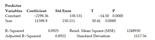 Interpret the estimated slope of the regression line.
A) For every 1-carat increase in the size of a diamond, we estimate that the price of the diamond will increase by $11,598.90.
B) For every 1-carat increase in the size of a diamond, we estimate that the price of the diamond will decrease by $2298.36.
C) For every $1 decrease in the price of the diamond, we estimate that the size of the diamond will increase by 11,598.9 carats.
D) For every 2298.36-carat decrease in the size of a diamond, we estimate that the price of the diamond will increase by $11,598.90.
Interpret the estimated slope of the regression line.A) For every 1-carat increase in the size of a diamond, we estimate that the price of the diamond will increase by $11,598.90.
B) For every 1-carat increase in the size of a diamond, we estimate that the price of the diamond will decrease by $2298.36.
C) For every $1 decrease in the price of the diamond, we estimate that the size of the diamond will increase by 11,598.9 carats.
D) For every 2298.36-carat decrease in the size of a diamond, we estimate that the price of the diamond will increase by $11,598.90.
Question
Question
Question
Question
A company keeps extensive records on its new salespeople on the premise that sales should increase with experience. A random sample of seven new salespeople produced the data on experience and sales shown in the table. 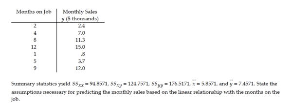
Question
If a least squares line were determined for the data set in each scattergram, which would have the smallest variance? 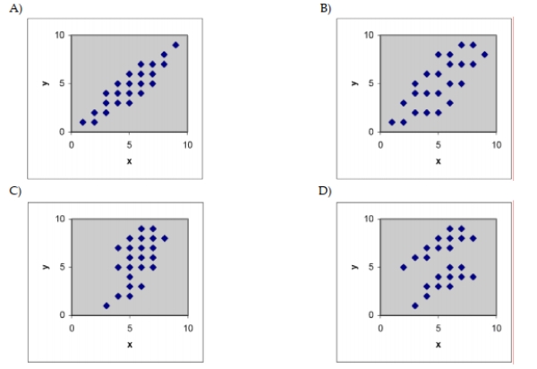
Question
Consider the data set shown below. Find the 95% confidence interval for the slope of the regression line. 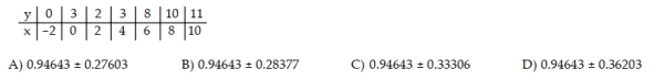
Question
Question
Question
Consider the following pairs of measurements: 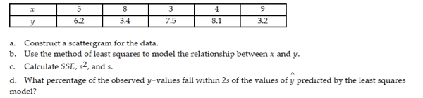 11.4 Assessing the Utility of the Model: Making Inferences about the Slope β1 1 Construct Confidence Interval for β1
11.4 Assessing the Utility of the Model: Making Inferences about the Slope β1 1 Construct Confidence Interval for β1 Question
Question
Question
Question
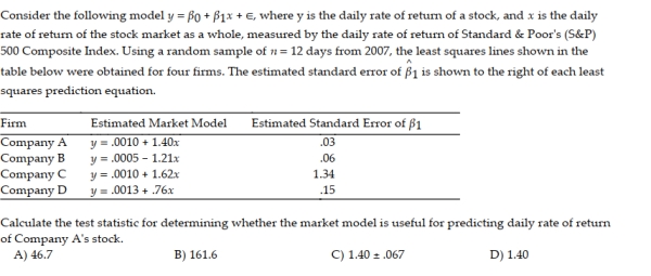
A large national bank charges local companies for using their services. A bank official reported the results of a regression analysis designed to predict the bank's charges (y), measured in dollars per month, for services rendered to local companies. One independent variable used to predict service charge to a company is the company's sales revenue (x), measured in $ million. Data for 21 companies who use the bank's services were used to fit the model 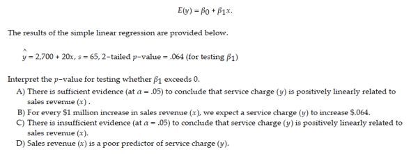
Question
A breeder of Thoroughbred horses wishes to model the relationship between the gestation period and the length of life of a horse. The breeder believes that the two variables may follow a linear trend. The information in the table was supplied to the breeder from various thoroughbred stables across the state. 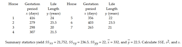
Question
Question
An academic advisor wants to predict the typical starting salary of a graduate at a top business school using the GMAT score of the school as a predictor variable. A simple linear regression of SALARY versus GMAT using 25 data points is shown below. 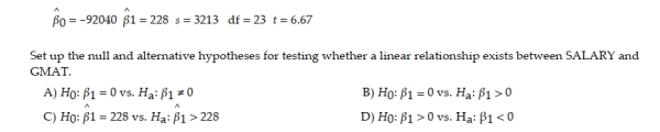
Question
Question
In a study of feeding behavior, zoologists recorded the number of grunts of a warthog feeding by a lake in the 15 minute period following the addition of food. The data showing the number of grunts and the age of the warthog (in days) are listed below: 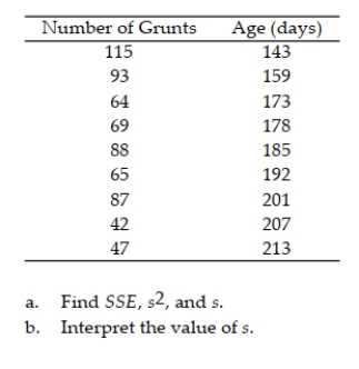
Question
Question
Question
Construct a 95% confidence interval for 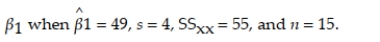
Question
Is the number of games won by a major league baseball team in a season related to the team's batting average? Data from 14 teams were collected and the summary statistics yield: 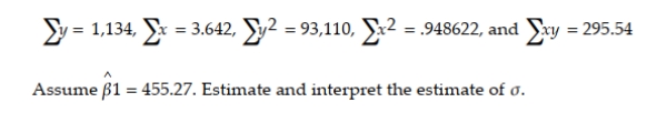
Question
A county real estate appraiser wants to develop a statistical model to predict the appraised value of houses in a section of the county called East Meadow. One of the many variables thought to be an important predictor of appraised value is the number of rooms in the house. Consequently, the appraiser decided to fit the simple linear regression model: 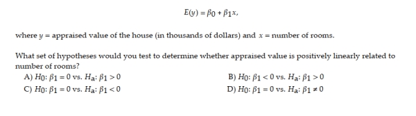
Question
Construct a 90% confidence interval for 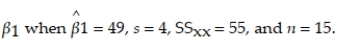
Question
Question
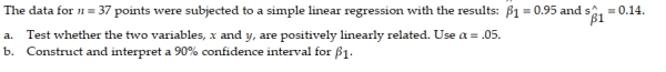
Consider the following pairs of observations: 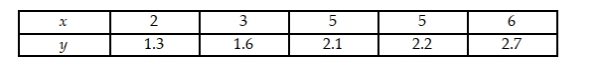 a. Construct a scattergram for the data. Does the scattergram suggest that y is positively linearly related to x? b. Find the slope of the least squares line for the data and test whether the data provide sufficient evidence that y is positively linearly related to x. Use α = .05.
a. Construct a scattergram for the data. Does the scattergram suggest that y is positively linearly related to x? b. Find the slope of the least squares line for the data and test whether the data provide sufficient evidence that y is positively linearly related to x. Use α = .05. Question
Consider the following pairs of observations: 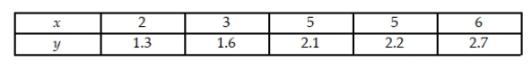 Find and interpret the value of the coefficient of correlation.
Find and interpret the value of the coefficient of correlation. Question
Question
Question
What is the relationship between diamond price and carat size? 307 diamonds were sampled and a straight-line relationship was hypothesized between y = diamond price (in dollars) and x = size of the diamond (in carats). The simple linear regression for the analysis is shown below: Least Squares Linear Regression of PRICE 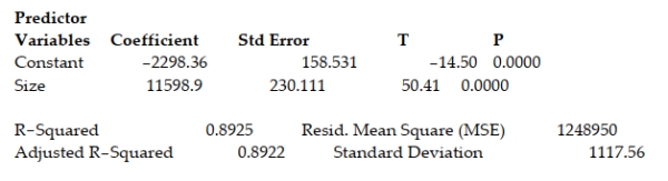 Which of the following conclusions is correct when testing to determine if the size of the diamond is a useful positive linear predictor of the price of a diamond?
A) There is insufficient evidence to indicate that the size of the diamond is a useful positive linear predictor of the price of a diamond when testing at α = 0.05.
B) There is sufficient evidence to indicate that the size of the diamond is a useful positive linear predictor of the price of a diamond when testing at α = 0.05.
C) There is insufficient evidence to indicate that the price of the diamond is a useful positive linear predictor of the size of a diamond when testing at α = 0.05.
D) The sample size is too small to make any conclusions regarding the regression line.
Which of the following conclusions is correct when testing to determine if the size of the diamond is a useful positive linear predictor of the price of a diamond?A) There is insufficient evidence to indicate that the size of the diamond is a useful positive linear predictor of the price of a diamond when testing at α = 0.05.
B) There is sufficient evidence to indicate that the size of the diamond is a useful positive linear predictor of the price of a diamond when testing at α = 0.05.
C) There is insufficient evidence to indicate that the price of the diamond is a useful positive linear predictor of the size of a diamond when testing at α = 0.05.
D) The sample size is too small to make any conclusions regarding the regression line.
Question
In a study of feeding behavior, zoologists recorded the number of grunts of a warthog feeding by a lake in the 15 minute period following the addition of food. The data showing the number of grunts and and the age of the warthog (in days) are listed below: 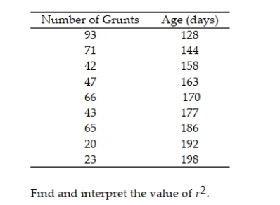
Question
Question
Question
Question
Question
In a study of feeding behavior, zoologists recorded the number of grunts of a warthog feeding by a lake in the 15 minute period following the addition of food. The data showing the number of grunts and and the age of the warthog (in days) are listed below: 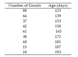 Find and interpret the value of r.
Find and interpret the value of r. Question
Question
A breeder of Thoroughbred horses wishes to model the relationship between the gestation period and the length of life of a horse. The breeder believes that the two variables may follow a linear trend. The information in the table was supplied to the breeder from various thoroughbred stables across the state. 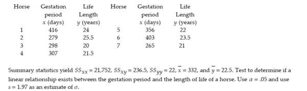
Question
Question
Is the number of games won by a major league baseball team in a season related to the team's batting average? Data from 14 teams were collected and the summary statistics yield: 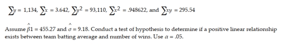
Question
Question
Question
To investigate the relationship between yield of potatoes, y, and level of fertilizer application, x, a researcher divides a field into eight plots of equal size and applies differing amounts of fertilizer to each. The yield of potatoes (in pounds) and the fertilizer application (in pounds) are recorded for each plot. The data are as follows: 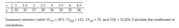
Question
A realtor collected the following data for a random sample of ten homes that recently sold in her area. 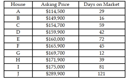 a. Construct a scattergram for the data. b. Find the least squares line for the data and plot the line on your scattergram. c. Test whether the number of days on the market, y, is positively linearly related to the asking price, x. Use α = .05.
a. Construct a scattergram for the data. b. Find the least squares line for the data and plot the line on your scattergram. c. Test whether the number of days on the market, y, is positively linearly related to the asking price, x. Use α = .05. Question

Unlock Deck
Sign up to unlock the cards in this deck!
Unlock Deck
Unlock Deck
1/111
Play
Full screen (f)
Deck 11: Simple Linear Regression
1
Is the number of games won by a major league baseball team in a season related to the team's batting average? Data from 14 teams were collected and the summary statistics yield: Find the least squares prediction equation for predicting the number of games won, y, using a straight-line relationship with the team's batting average, x.
Find the least squares prediction equation for predicting the number of games won, y, using a straight-line relationship with the team's batting average, x.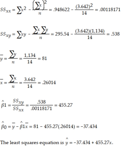
2
To investigate the relationship between yield of potatoes, y, and level of fertilizer application, x, a researcher divides a field into eight plots of equal size and applies differing amounts of fertilizer to each. The yield of potatoes (in pounds) and the fertilizer application (in pounds) are recorded for each plot. The data are as follows:
β1 = SSSSxyxx = 10.525 ≈ 2.3810
β^0 = y - β1x = 31 - 2.3810(2.75) = 24.4523
The least squares prediction equation is y^ = 24.4523 + 2.3810x
β^0 = y - β1x = 31 - 2.3810(2.75) = 24.4523
The least squares prediction equation is y^ = 24.4523 + 2.3810x
3
(0, 6) and (6, 0)
A
4
Unlock Deck
Unlock for access to all 111 flashcards in this deck.
Unlock Deck
k this deck
5
(-6, 0) and (-3, -1)
Unlock Deck
Unlock for access to all 111 flashcards in this deck.
Unlock Deck
k this deck
6
(2, -6) and (-1, 3)
Unlock Deck
Unlock for access to all 111 flashcards in this deck.
Unlock Deck
k this deck
7
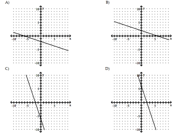
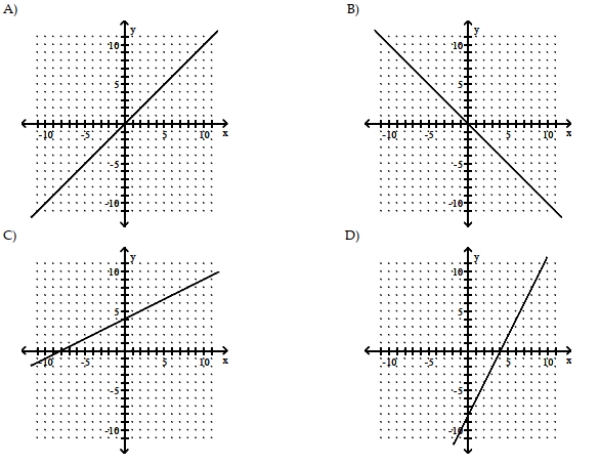
Plot the line y = 4 - 2x. Then give the slope and y-intercept of the line.
Unlock Deck
Unlock for access to all 111 flashcards in this deck.
Unlock Deck
k this deck
8
(-7, -6) and (-1, -7)
Unlock Deck
Unlock for access to all 111 flashcards in this deck.
Unlock Deck
k this deck
9
Unlock Deck
Unlock for access to all 111 flashcards in this deck.
Unlock Deck
k this deck
10
Consider the data set shown below. Find the estimate of the slope of the least squares regression line.
A) 1.5
B) 0.94643
C) 1.49045
D) 0.9003
A) 1.5
B) 0.94643
C) 1.49045
D) 0.9003
Unlock Deck
Unlock for access to all 111 flashcards in this deck.
Unlock Deck
k this deck
11
(-8, -8) and (4, 4)
Unlock Deck
Unlock for access to all 111 flashcards in this deck.
Unlock Deck
k this deck
12
Plot the line y = 3x. Then give the slope and y-intercept of the line.
Unlock Deck
Unlock for access to all 111 flashcards in this deck.
Unlock Deck
k this deck
13
Consider the following pairs of measurements: a. Construct a scattergram for the data. b. What does the scattergram suggest about the relationship between x and y? c. Find the least squares estimates of β0 and β1. d. Plot the least squares line on your scattergram. Does the line appear to fit the data well?
a. Construct a scattergram for the data. b. What does the scattergram suggest about the relationship between x and y? c. Find the least squares estimates of β0 and β1. d. Plot the least squares line on your scattergram. Does the line appear to fit the data well? Unlock Deck
Unlock for access to all 111 flashcards in this deck.
Unlock Deck
k this deck
14
In a study of feeding behavior, zoologists recorded the number of grunts of a warthog feeding by a lake in the 15 minute period following the addition of food. The data showing the number of grunts and and the age of the warthog (in days) are listed below:
Unlock Deck
Unlock for access to all 111 flashcards in this deck.
Unlock Deck
k this deck
15
A county real estate appraiser wants to develop a statistical model to predict the appraised value of houses in a section of the county called East Meadow. One of the many variables thought to be an important predictor of appraised value is the number of rooms in the house. Consequently, the appraiser decided to fit the simple linear regression model:
Unlock Deck
Unlock for access to all 111 flashcards in this deck.
Unlock Deck
k this deck
16
In a comprehensive road test for new car models, one variable measured is the time it takes the car to accelerate from 0 to 60 miles per hour. To model acceleration time, a regression analysis is conducted on a random sample of 129 new cars. TIME60: y = Elapsed time (in seconds) from 0 mph to 60 mph MAX: x = Maximum speed attained (miles per hour)
Unlock Deck
Unlock for access to all 111 flashcards in this deck.
Unlock Deck
k this deck
17
The probabilistic model allows the E(y) values to fall around the regression line while the actual values of y must fall on the line.
Unlock Deck
Unlock for access to all 111 flashcards in this deck.
Unlock Deck
k this deck
18
Plot the line y = 1.5 + .5x. Then give the slope and y-intercept of the line.
Unlock Deck
Unlock for access to all 111 flashcards in this deck.
Unlock Deck
k this deck
19
Is there a relationship between the raises administrators at County University receive and their performance on the job? A faculty group wants to determine whether job rating (x) is a useful linear predictor of raise (y). Consequently, the group considered the linear regression model
Unlock Deck
Unlock for access to all 111 flashcards in this deck.
Unlock Deck
k this deck
20
Consider the data set shown below. Find the estimate of the y-intercept of the least squares regression line.
A) 1.5
B) 0.94643
C) 1.49045
D) 0.9003
A) 1.5
B) 0.94643
C) 1.49045
D) 0.9003
Unlock Deck
Unlock for access to all 111 flashcards in this deck.
Unlock Deck
k this deck
21
Suppose you fit a least squares line to 25 data points and the calculated value of SSE is 0.42.
Unlock Deck
Unlock for access to all 111 flashcards in this deck.
Unlock Deck
k this deck
22
What is the relationship between diamond price and carat size? 307 diamonds were sampled and a straight-line relationship was hypothesized between y = diamond price (in dollars) and x = size of the diamond (in carats). The simple linear regression for the analysis is shown below: Least Squares Linear Regression of PRICE Which of the following assumptions is not stated correctly?
A) The probability distribution of ε is normal.
B) The mean of the probability distribution of ε is 0.
C) The variance of the probability distribution of ε is constant for all settings of the independent variable.
D) The values of ε associated with any two observations are dependent on one another.
Which of the following assumptions is not stated correctly?A) The probability distribution of ε is normal.
B) The mean of the probability distribution of ε is 0.
C) The variance of the probability distribution of ε is constant for all settings of the independent variable.
D) The values of ε associated with any two observations are dependent on one another.
Unlock Deck
Unlock for access to all 111 flashcards in this deck.
Unlock Deck
k this deck
23
Is there a relationship between the raises administrators at State University receive and their performance on the job? A faculty group wants to determine whether job rating (x) is a useful linear predictor of raise (y). Consequently, the group considered the straight-line regression model
Using the method of least squares, the faculty group obtained the following prediction equation:
Interpret the estimated y-intercept of the line.
A) For an administrator who receives a rating of zero, we estimate his or her raise to be $14,000.
B) The base administrator raise at State University is $14,000.
C) For a 1-point increase in an administrator's rating, we estimate the administrator's raise to increase $14,000.
D) There is no practical interpretation, since rating of 0 is nonsensical and outside the range of the sample data.
Unlock Deck
Unlock for access to all 111 flashcards in this deck.
Unlock Deck
k this deck
24
The Method of Least Squares specifies that the regression line has an average error of 0 and has an SSE that is minimized.
Unlock Deck
Unlock for access to all 111 flashcards in this deck.
Unlock Deck
k this deck
25
A study of the top 75 MBA programs attempted to predict the average starting salary (in $1000's) of graduates of the program based on the amount of tuition (in $1000's) charged by the program. The results of a simple linear regression analysis are shown below: Least Squares Linear Regression of Salary Predictor
R-Squared Resid. Mean Square (MSE)
Adjusted R-Squared Standard Deviation Interpret the estimated slope of the regression line.
A) For every $1000 increase in the tuition charged by the MBA program, we estimate that the average starting salary will decrease by $1474.94.
B) For every $1000 increase in the tuition charged by the MBA program, we estimate that the average starting salary will increase by $1474.94.
C) For every $1474.94 increase in the tuition charged by the MBA program, we estimate that the average starting salary will increase by $18,184.90.
D) For every $1000 increase in the average starting salary, we estimate that the tuition charged by the MBA program will increase by $1474.94.
Unlock Deck
Unlock for access to all 111 flashcards in this deck.
Unlock Deck
k this deck
26
An academic advisor wants to predict the typical starting salary of a graduate at a top business school using the GMAT score of the school as a predictor variable. A simple linear regression of SALARY versus GMAT was created from a set of 25 data points. Which of the following is not an assumption required for the simple linear regression analysis to be valid?
A) SALARY is independent of GMAT.
B) The errors of predicting SALARY are normally distributed.
C) The errors of predicting SALARY have a mean of 0.
D) The errors of predicting SALARY have a variance that is constant for any given value of GMAT.
A) SALARY is independent of GMAT.
B) The errors of predicting SALARY are normally distributed.
C) The errors of predicting SALARY have a mean of 0.
D) The errors of predicting SALARY have a variance that is constant for any given value of GMAT.
Unlock Deck
Unlock for access to all 111 flashcards in this deck.
Unlock Deck
k this deck
27
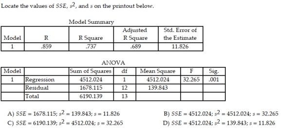
Consider the data set shown below. Find the standard deviation of the least squares regression line.
A) 1.5
B) 0.94643
C) 1.49045
D) 0.9003
A) 1.5
B) 0.94643
C) 1.49045
D) 0.9003
Unlock Deck
Unlock for access to all 111 flashcards in this deck.
Unlock Deck
k this deck
28
What is the relationship between diamond price and carat size? 307 diamonds were sampled (ranging in size from 0.18 to 1.1 carats) and a straight-line relationship was hypothesized between y = diamond price (in dollars) and x = size of the diamond (in carats). The simple linear regression for the analysis is shown below: Least Squares Linear Regression of PRICE Interpret the estimated y-intercept of the regression line.
A) When a diamond is 0 carats in size, we estimate the price of the diamond to be $11,598.90.
B) When a diamond is 0 carats in size, we estimate the price of the diamond to be $2298.36.
C) When a diamond is 11598.9 carats in size, we estimate the price of the diamond to be $2298.36.
D) No practical interpretation of the y-intercept exists since a diamond of 0 carats cannot exist and falls outside the range of the carat sizes sampled.
Interpret the estimated y-intercept of the regression line.A) When a diamond is 0 carats in size, we estimate the price of the diamond to be $11,598.90.
B) When a diamond is 0 carats in size, we estimate the price of the diamond to be $2298.36.
C) When a diamond is 11598.9 carats in size, we estimate the price of the diamond to be $2298.36.
D) No practical interpretation of the y-intercept exists since a diamond of 0 carats cannot exist and falls outside the range of the carat sizes sampled.
Unlock Deck
Unlock for access to all 111 flashcards in this deck.
Unlock Deck
k this deck
29
Unlock Deck
Unlock for access to all 111 flashcards in this deck.
Unlock Deck
k this deck
30
A large national bank charges local companies for using its services. A bank official reported the results of a regression analysis designed to predict the bank's charges (y), measured in dollars per month, for services rendered to local companies. One independent variable used to predict the service charge to a company is the company's sales revenue (x), measured in $ million. Data for 21 companies who use the bank's services were used to fit the model
The results of the simple linear regression are provided below.
Interpret the estimate of , the -intercept of the line.
A) There is no practical interpretation since a sales revenue of $0 is a nonsensical value.
B) All companies will be charged at least $2,700 by the bank.
C) About 95% of the observed service charges fall within $2,700 of the least squares line.
D) For every $1 million increase in sales revenue, we expect a service charge to increase $2,700.
Unlock Deck
Unlock for access to all 111 flashcards in this deck.
Unlock Deck
k this deck
31
What is the relationship between diamond price and carat size? 307 diamonds were sampled and a straight-line relationship was hypothesized between y = diamond price (in dollars) and x = size of the diamond (in carats). The simple linear regression for the analysis is shown below: Least Squares Linear Regression of PRICE Interpret the standard deviation of the regression model.
A) We can explain 89.25% of the variation in the sampled diamond prices around their mean using the size of the diamond in a linear model.
B) We expect most of the sampled diamond prices to fall within $1117.56 of their least squares predicted values.
C) We expect most of the sampled diamond prices to fall within $2235.12 of their least squares predicted values.
D) For every 1-carat increase in the size of a diamond, we estimate that the price of the diamond will increase by $1117.56.
Interpret the standard deviation of the regression model.A) We can explain 89.25% of the variation in the sampled diamond prices around their mean using the size of the diamond in a linear model.
B) We expect most of the sampled diamond prices to fall within $1117.56 of their least squares predicted values.
C) We expect most of the sampled diamond prices to fall within $2235.12 of their least squares predicted values.
D) For every 1-carat increase in the size of a diamond, we estimate that the price of the diamond will increase by $1117.56.
Unlock Deck
Unlock for access to all 111 flashcards in this deck.
Unlock Deck
k this deck
32
State the four basic assumptions about the general form of the probability distribution of the random error ε.
Unlock Deck
Unlock for access to all 111 flashcards in this deck.
Unlock Deck
k this deck
33
Unlock Deck
Unlock for access to all 111 flashcards in this deck.
Unlock Deck
k this deck
34
Suppose you fit a least squares line to 22 data points and the calculated value of SSE is .678. a. Find s2, the estimator of σ2. b. Find s, the estimator of σ. c. What is the largest deviation you might expect between any one of the 22 points and the least squares line?
Unlock Deck
Unlock for access to all 111 flashcards in this deck.
Unlock Deck
k this deck
35
What is the relationship between diamond price and carat size? 307 diamonds were sampled and a straight-line relationship was hypothesized between y = diamond price (in dollars) and x = size of the diamond (in carats). The simple linear regression for the analysis is shown below: Least Squares Linear Regression of PRICE Interpret the estimated slope of the regression line.
A) For every 1-carat increase in the size of a diamond, we estimate that the price of the diamond will increase by $11,598.90.
B) For every 1-carat increase in the size of a diamond, we estimate that the price of the diamond will decrease by $2298.36.
C) For every $1 decrease in the price of the diamond, we estimate that the size of the diamond will increase by 11,598.9 carats.
D) For every 2298.36-carat decrease in the size of a diamond, we estimate that the price of the diamond will increase by $11,598.90.
Interpret the estimated slope of the regression line.A) For every 1-carat increase in the size of a diamond, we estimate that the price of the diamond will increase by $11,598.90.
B) For every 1-carat increase in the size of a diamond, we estimate that the price of the diamond will decrease by $2298.36.
C) For every $1 decrease in the price of the diamond, we estimate that the size of the diamond will increase by 11,598.9 carats.
D) For every 2298.36-carat decrease in the size of a diamond, we estimate that the price of the diamond will increase by $11,598.90.
Unlock Deck
Unlock for access to all 111 flashcards in this deck.
Unlock Deck
k this deck
36
A county real estate appraiser wants to develop a statistical model to predict the appraised value of houses in a section of the county called East Meadow. One of the many variables thought to be an important predictor of appraised value is the number of rooms in the house. Consequently, the appraiser decided to fit the simple linear regression model:
where appraised value of the house (in thousands of dollars) and number of rooms. Using data collected for a sample of houses in East Meadow, the following restults were obtained:
Give a practical interpretation of the estimate of the slope of the least squares line.
A) For each additional room in the house, we estimate the appraised value to increase $21,660.
B) For each additional room in the house, we estimate the appraised value to increase $74,800.
C) For each additional dollar of appraised value, we estimate the number of rooms in the house to increase by 21.66.
D) For a house with 0 rooms, we estimate the appraised value to be $74,800.
Unlock Deck
Unlock for access to all 111 flashcards in this deck.
Unlock Deck
k this deck
37
Is there a relationship between the raises administrators at State University receive and their performance on the job? A faculty group wants to determine whether job rating (x) is a useful linear predictor of raise (y). Consequently, the group considered the straight-line regression model
Using the method of least squares, the faculty group obtained the following prediction equation:
Interpret the estimated slope of the line.
A) For a 1-point increase in an administrator's rating, we estimate the administrator's raise to decrease $2,000.
B) For a 1-point increase in an administrator's rating, we estimate the administrator's raise to increase $2,000.
C) For an administrator with a rating of 1.0, we estimate his/her raise to be $2,000.
D) For a $1 increase in an administrator's raise, we estimate the administrator's rating to decrease 2,000 points.
Unlock Deck
Unlock for access to all 111 flashcards in this deck.
Unlock Deck
k this deck
38
A county real estate appraiser wants to develop a statistical model to predict the appraised value of houses in a section of the county called East Meadow. One of the many variables thought to be an important predictor of appraised value is the number of rooms in the house. Consequently, the appraiser decided to fit the simple linear regression model:
where appraised value of the house (in thousands of dollars) and number of rooms. Using data collected for a sample of houses in East Meadow, the following results were obtained:
Give a practical interpretation of the estimate of the y-intercept of the least squares line.
A) There is no practical interpretation, since a house with 0 rooms is nonsensical.
B) For each additional room in the house, we estimate the appraised value to increase $74,800.
C) For each additional room in the house, we estimate the appraised value to increase $19,720.
D) We estimate the base appraised value for any house to be $74,800.
Unlock Deck
Unlock for access to all 111 flashcards in this deck.
Unlock Deck
k this deck
39
A company keeps extensive records on its new salespeople on the premise that sales should increase with experience. A random sample of seven new salespeople produced the data on experience and sales shown in the table.
Unlock Deck
Unlock for access to all 111 flashcards in this deck.
Unlock Deck
k this deck
40
If a least squares line were determined for the data set in each scattergram, which would have the smallest variance?
Unlock Deck
Unlock for access to all 111 flashcards in this deck.
Unlock Deck
k this deck
41
Consider the data set shown below. Find the 95% confidence interval for the slope of the regression line.
Unlock Deck
Unlock for access to all 111 flashcards in this deck.
Unlock Deck
k this deck
42
The dean of the Business School at a small Florida college wishes to determine whether the grade -point average (GPA) of a graduating student can be used to predict the graduate's starting salary. More specifically, the dean wants to know whether higher GPAs lead to higher starting salaries. Records for 23 of last year's Business School graduates are selected at random, and data on GPA (x) and starting salary (y, in $thousands) for each graduate were used to fit the model . The value of the test statistic for testing ?1 is 17.169. Select the proper conclusion.
A) There is sufficient evidence (at ? = .05) to conclude that GPA is positively linearly related to starting salary.
B) There is insufficient evidence (at ? = .05) to conclude that GPA is positively linearly related to starting salary.
C) There is insufficient evidence (at ? = .10) to conclude that GPA is a useful linear predictor of starting salary.
D) At any reasonable ?, there is no relationship between GPA and starting salary.
Unlock Deck
Unlock for access to all 111 flashcards in this deck.
Unlock Deck
k this deck
43
Unlock Deck
Unlock for access to all 111 flashcards in this deck.
Unlock Deck
k this deck
44
Consider the following pairs of measurements: 11.4 Assessing the Utility of the Model: Making Inferences about the Slope β1 1 Construct Confidence Interval for β1
11.4 Assessing the Utility of the Model: Making Inferences about the Slope β1 1 Construct Confidence Interval for β1 Unlock Deck
Unlock for access to all 111 flashcards in this deck.
Unlock Deck
k this deck
45
Unlock Deck
Unlock for access to all 111 flashcards in this deck.
Unlock Deck
k this deck
46
Unlock Deck
Unlock for access to all 111 flashcards in this deck.
Unlock Deck
k this deck
47
A manufacturer of boiler drums wants to use regression to predict the number of man-hours needed to erect drums in the future. The manufacturer collected a random sample of 35 boilers and measured the following two variables: MANHRS: Number of man-hours required to erect the drum
PRESSURE: Boiler design pressure (pounds per square inch, i.e., )
The simple linear model was fit to the data. A printout for the analysis appears below:
UNWEIGHTED LEAST SQUARES LINEAR REGRESSION OF MANHRS
Fill in the blank. At ? =.01, there is ____________ between man-hours and pressure.
A) insufficient evidence of a positive linear relationship
B) sufficient evidence of a positive linear relationship
C) sufficient evidence of a negative linear relationship
D) sufficient evidence of a linear relationship
Unlock Deck
Unlock for access to all 111 flashcards in this deck.
Unlock Deck
k this deck
48
A large national bank charges local companies for using their services. A bank official reported the results of a regression analysis designed to predict the bank's charges (y), measured in dollars per month, for services rendered to local companies. One independent variable used to predict service charge to a company is the company's sales revenue (x), measured in $ million. Data for 21 companies who use the bank's services were used to fit the model
Unlock Deck
Unlock for access to all 111 flashcards in this deck.
Unlock Deck
k this deck
49
A breeder of Thoroughbred horses wishes to model the relationship between the gestation period and the length of life of a horse. The breeder believes that the two variables may follow a linear trend. The information in the table was supplied to the breeder from various thoroughbred stables across the state.
Unlock Deck
Unlock for access to all 111 flashcards in this deck.
Unlock Deck
k this deck
50
In a comprehensive road test on new car models, one variable measured is the time it takes a car to accelerate from 0 to 60 miles per hour. To model acceleration time, a regression analysis is conducted on a random sample of 129 new cars. TIME60: Elapsed time (in seconds) from to
MAX: Maximum speed attained (miles per hour)
The simple linear model was fit to the data. Computer printouts for the analysis are given below:
NWEIGHTED LEAST SQUARES LINEAR REGRESSION OF TIME60
CASES INCLUDED 129 MISSING CASES 0 Fill in the blank: "At ? =.05, there is ________________ between maximum speed and acceleration time."
A) sufficient evidence of a negative linear relationship
B) insufficient evidence of a negative linear relationship
C) sufficient evidence of a positive linear relationship
D) insufficient evidence of a linear relationship
Unlock Deck
Unlock for access to all 111 flashcards in this deck.
Unlock Deck
k this deck
51
An academic advisor wants to predict the typical starting salary of a graduate at a top business school using the GMAT score of the school as a predictor variable. A simple linear regression of SALARY versus GMAT using 25 data points is shown below.
Unlock Deck
Unlock for access to all 111 flashcards in this deck.
Unlock Deck
k this deck
52
Unlock Deck
Unlock for access to all 111 flashcards in this deck.
Unlock Deck
k this deck
53
In a study of feeding behavior, zoologists recorded the number of grunts of a warthog feeding by a lake in the 15 minute period following the addition of food. The data showing the number of grunts and the age of the warthog (in days) are listed below:
Unlock Deck
Unlock for access to all 111 flashcards in this deck.
Unlock Deck
k this deck
54
A county real estate appraiser wants to develop a statistical model to predict the appraised value of houses in a section of the county called East Meadow. One of the many variables thought to be an important predictor of appraised value is the number of rooms in the house. Consequently, the appraiser decided to fit the simple linear regression model:
where appraised value of the house (in thousands of dollars) and number of rooms. Using data collected for a sample of houses in East Meadow, the following results were obtained:
Give a practical interpretation of the estimate of ?, the standard deviation of the random error term in the model.
A) We expect to predict the appraised value of an East Meadow house to within about $58,000 of its true value.
B) We expect to predict the appraised value of an East Meadow house to within about $29,000 of its true value.
C) We expect 95% of the observed appraised values to lie on the least squares line.
D) About 29% of the total variation in the sample of y-values can be explained by the linear relationship between appraised value and number of rooms.
Unlock Deck
Unlock for access to all 111 flashcards in this deck.
Unlock Deck
k this deck
55
A large national bank charges local companies for using their services. A bank official reported the results of a regression analysis designed to predict the bank's charges (y), measured in dollars per month, for services rendered to local companies. One independent variable used to predict service charge to a company is the company's sales revenue (x), measured in $ million. Data for 21 companies who use the bank's services were used to fit the model Suppose a 95% confidence interval for ?1 is (15, 25). Interpret the interval.
A) We are 95% confident that service charge (y) will increase between $15 and $25 for every $1 million increase in sales revenue (x).
B) We are 95% confident that the mean service charge will fall between $15 and $25 per month.
C) We are 95% confident that sales revenue (x) will increase between $15 and $25 million for every $1 increase in service charge (y).
D) We are 95% confident that service charge (y) will decrease between $15 and $25 for every $1 million increase in sales revenue (x).
Unlock Deck
Unlock for access to all 111 flashcards in this deck.
Unlock Deck
k this deck
56
Construct a 95% confidence interval for
Unlock Deck
Unlock for access to all 111 flashcards in this deck.
Unlock Deck
k this deck
57
Is the number of games won by a major league baseball team in a season related to the team's batting average? Data from 14 teams were collected and the summary statistics yield:
Unlock Deck
Unlock for access to all 111 flashcards in this deck.
Unlock Deck
k this deck
58
A county real estate appraiser wants to develop a statistical model to predict the appraised value of houses in a section of the county called East Meadow. One of the many variables thought to be an important predictor of appraised value is the number of rooms in the house. Consequently, the appraiser decided to fit the simple linear regression model:
Unlock Deck
Unlock for access to all 111 flashcards in this deck.
Unlock Deck
k this deck
59
Construct a 90% confidence interval for
Unlock Deck
Unlock for access to all 111 flashcards in this deck.
Unlock Deck
k this deck
60
The dean of the Business School at a small Florida college wishes to determine whether the grade -point average (GPA) of a graduating student can be used to predict the graduate's starting salary. More specifically, the dean wants to know whether higher GPAs lead to higher starting salaries. Records for 23 of last year's Business School graduates are selected at random, and data on GPA (x) and starting salary (y, in $thousands) for each graduate were used to fit the model
The results of the simple linear regression are provided below.
Compute an estimate of ?, the standard deviation of the random error term.
A) 0.219
B) 1.0075
C) .689
D) .048
The results of the simple linear regression are provided below.
Compute an estimate of ?, the standard deviation of the random error term.
A) 0.219
B) 1.0075
C) .689
D) .048
Unlock Deck
Unlock for access to all 111 flashcards in this deck.
Unlock Deck
k this deck
61
Consider the following pairs of observations: a. Construct a scattergram for the data. Does the scattergram suggest that y is positively linearly related to x? b. Find the slope of the least squares line for the data and test whether the data provide sufficient evidence that y is positively linearly related to x. Use α = .05.
a. Construct a scattergram for the data. Does the scattergram suggest that y is positively linearly related to x? b. Find the slope of the least squares line for the data and test whether the data provide sufficient evidence that y is positively linearly related to x. Use α = .05. Unlock Deck
Unlock for access to all 111 flashcards in this deck.
Unlock Deck
k this deck
62
Consider the following pairs of observations: Find and interpret the value of the coefficient of correlation.
Find and interpret the value of the coefficient of correlation. Unlock Deck
Unlock for access to all 111 flashcards in this deck.
Unlock Deck
k this deck
63
Consider the data set shown below. Find the coefficient of determination for the simple linear regression model.
A) 0.9003
B) 0.8804
C) 0.9489
D) 0.9383
A) 0.9003
B) 0.8804
C) 0.9489
D) 0.9383
Unlock Deck
Unlock for access to all 111 flashcards in this deck.
Unlock Deck
k this deck
64
A study of the top 75 MBA programs attempted to predict the average starting salary (in $1000's) of graduates of the program based on the amount of tuition (in $1000's) charged by the program. The results of a simple linear regression analysis are shown below: Least Squares Linear Regression of Salary Predictor
Fill in the blank. At ? = 0.05, there is _________________ between the amount of tuition charged by an MBA program and the average starting salary of graduates of the program.
A) …sufficient evidence of a negative linear relationship…
B) …insufficient evidence of a positive linear relationship…
C) …sufficient evidence of a positive linear relationship…
Unlock Deck
Unlock for access to all 111 flashcards in this deck.
Unlock Deck
k this deck
65
What is the relationship between diamond price and carat size? 307 diamonds were sampled and a straight-line relationship was hypothesized between y = diamond price (in dollars) and x = size of the diamond (in carats). The simple linear regression for the analysis is shown below: Least Squares Linear Regression of PRICE Which of the following conclusions is correct when testing to determine if the size of the diamond is a useful positive linear predictor of the price of a diamond?
A) There is insufficient evidence to indicate that the size of the diamond is a useful positive linear predictor of the price of a diamond when testing at α = 0.05.
B) There is sufficient evidence to indicate that the size of the diamond is a useful positive linear predictor of the price of a diamond when testing at α = 0.05.
C) There is insufficient evidence to indicate that the price of the diamond is a useful positive linear predictor of the size of a diamond when testing at α = 0.05.
D) The sample size is too small to make any conclusions regarding the regression line.
Which of the following conclusions is correct when testing to determine if the size of the diamond is a useful positive linear predictor of the price of a diamond?A) There is insufficient evidence to indicate that the size of the diamond is a useful positive linear predictor of the price of a diamond when testing at α = 0.05.
B) There is sufficient evidence to indicate that the size of the diamond is a useful positive linear predictor of the price of a diamond when testing at α = 0.05.
C) There is insufficient evidence to indicate that the price of the diamond is a useful positive linear predictor of the size of a diamond when testing at α = 0.05.
D) The sample size is too small to make any conclusions regarding the regression line.
Unlock Deck
Unlock for access to all 111 flashcards in this deck.
Unlock Deck
k this deck
66
In a study of feeding behavior, zoologists recorded the number of grunts of a warthog feeding by a lake in the 15 minute period following the addition of food. The data showing the number of grunts and and the age of the warthog (in days) are listed below:
Unlock Deck
Unlock for access to all 111 flashcards in this deck.
Unlock Deck
k this deck
67
A high value of the correlation coefficient r implies that a causal relationship exists between x and y.
Unlock Deck
Unlock for access to all 111 flashcards in this deck.
Unlock Deck
k this deck
68
Consider the data set shown below. Find the coefficient of correlation for between the variables x and y.
A) 0.9003
B) 0.8804
C) 0.9489
D) 0.9383
A) 0.9003
B) 0.8804
C) 0.9489
D) 0.9383
Unlock Deck
Unlock for access to all 111 flashcards in this deck.
Unlock Deck
k this deck
69
A study of the top 75 MBA programs attempted to predict the average starting salary (in $1000's) of graduates of the program based on the amount of tuition (in $1000's) charged by the program. We are told that the coefficient of correlation was calculated to be r = 0.7763. Use this information to calculate the test statistic that would be used to determine if a positive linear relationship exists between the two variables.
A) t = 10.52
B) t = 1.475
C) t = 1.760
D) t = 0.6027
A) t = 10.52
B) t = 1.475
C) t = 1.760
D) t = 0.6027
Unlock Deck
Unlock for access to all 111 flashcards in this deck.
Unlock Deck
k this deck
70
In team-teaching, two or more teachers lead a class. An researcher tested the use of team-teaching in mathematics education. Two of the variables measured on each sample of 177 mathematics teachers were years of teaching experience x and reported success rate y (measured as a percentage) of team-teaching mathematics classes. a. The researcher hypothesized that mathematics teachers with more years of experience will report higher perceived success rates in team-taught classes. State this hypothesis in terms of the parameter of a linear model relating x to y. b. The correlation coefficient for the sample data was reported as r = -0.3. Interpret this result. c. Does the value of r support the hypothesis? Test using α = .05.
Unlock Deck
Unlock for access to all 111 flashcards in this deck.
Unlock Deck
k this deck
71
In a study of feeding behavior, zoologists recorded the number of grunts of a warthog feeding by a lake in the 15 minute period following the addition of food. The data showing the number of grunts and and the age of the warthog (in days) are listed below: Find and interpret the value of r.
Find and interpret the value of r. Unlock Deck
Unlock for access to all 111 flashcards in this deck.
Unlock Deck
k this deck
72
In team-teaching, two or more teachers lead a class. A researcher tested the use of team-teaching in mathematics education. Two of the variables measured on each teacher in a sample of 169 mathematics teachers were years of teaching experience x and reported success rate y (measured as a percentage) of team-teaching mathematics classes. The correlation coefficient for the sample data was reported as r = -0.34. Interpret this result.
Unlock Deck
Unlock for access to all 111 flashcards in this deck.
Unlock Deck
k this deck
73
A breeder of Thoroughbred horses wishes to model the relationship between the gestation period and the length of life of a horse. The breeder believes that the two variables may follow a linear trend. The information in the table was supplied to the breeder from various thoroughbred stables across the state.
Unlock Deck
Unlock for access to all 111 flashcards in this deck.
Unlock Deck
k this deck
74
An academic advisor wants to predict the typical starting salary of a graduate at a top business school using the GMAT score of the school as a predictor variable. A simple linear regression of SALARY versus GMAT using 25 data points is shown below. Give a practical interpretation of r = .81.
A) There appears to be a positive correlation between SALARY and GMAT.
B) We estimate SALARY to increase 81% for every 1-point increase in GMAT.
C) 81% of the sample variation in SALARY can be explained by using GMAT in a straight -line model.
D) We can predict SALARY correctly 81% of the time using GMAT in a straight-line model.
Unlock Deck
Unlock for access to all 111 flashcards in this deck.
Unlock Deck
k this deck
75
Is the number of games won by a major league baseball team in a season related to the team's batting average? Data from 14 teams were collected and the summary statistics yield:
Unlock Deck
Unlock for access to all 111 flashcards in this deck.
Unlock Deck
k this deck
76
The coefficient of correlation is a useful measure of the linear relationship between two variables.
Unlock Deck
Unlock for access to all 111 flashcards in this deck.
Unlock Deck
k this deck
77
A low value of the correlation coefficient r implies that x and y are unrelated.
Unlock Deck
Unlock for access to all 111 flashcards in this deck.
Unlock Deck
k this deck
78
To investigate the relationship between yield of potatoes, y, and level of fertilizer application, x, a researcher divides a field into eight plots of equal size and applies differing amounts of fertilizer to each. The yield of potatoes (in pounds) and the fertilizer application (in pounds) are recorded for each plot. The data are as follows:
Unlock Deck
Unlock for access to all 111 flashcards in this deck.
Unlock Deck
k this deck
79
A realtor collected the following data for a random sample of ten homes that recently sold in her area. a. Construct a scattergram for the data. b. Find the least squares line for the data and plot the line on your scattergram. c. Test whether the number of days on the market, y, is positively linearly related to the asking price, x. Use α = .05.
a. Construct a scattergram for the data. b. Find the least squares line for the data and plot the line on your scattergram. c. Test whether the number of days on the market, y, is positively linearly related to the asking price, x. Use α = .05. Unlock Deck
Unlock for access to all 111 flashcards in this deck.
Unlock Deck
k this deck
80
A study of the top 75 MBA programs attempted to predict the average starting salary (in $1000's) of graduates of the program based on the amount of tuition (in $1000's) charged by the program. The results of a simple linear regression analysis are shown below: Least Squares Linear Regression of Salary Predictor
R-Squared Resid. Mean Square (MSE)
Adjusted R-Squared Standard Deviation In addition, we are told that the coefficient of correlation was calculated to be r = 0.7763. Interpret this result.
A) There is a fairly strong negative linear relationship between the amount of tuition charged and the average starting salary variables.
B) There is a fairly strong positive linear relationship between the amount of tuition charged and the average starting salary variables.
C) There is a very weak positive linear relationship between the amount of tuition charged and the average starting salary variables.
D) There is almost no linear relationship between the amount of tuition charged and the average starting salary variables.
Unlock Deck
Unlock for access to all 111 flashcards in this deck.
Unlock Deck
k this deck
Unlock Deck
Unlock for access to all 111 flashcards in this deck.


