Deck 12: Multiple Regression and Model Building
Full screen (f)
Question
Question
Question
A study of the top MBA programs attempted to predict the average starting salary (in $1000's) of graduates of the program based on the amount of tuition (in $1000's) charged by the program and the average GMAT score of the program's students. The results of a regression analysis based on a sample of 75 MBA programs is shown below: Least Squares Linear Regression of Salary 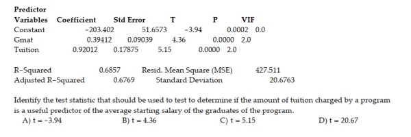
Question
Question
A study of the top MBA programs attempted to predict the average starting salary (in $1000's) of graduates of the program based on the amount of tuition (in $1000's) charged by the program and the average GMAT score of the program's students. The results of a regression analysis based on a sample of 75 MBA programs is shown below: Least Squares Linear Regression of Salary 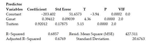 Interpret the coefficient for the tuition variable shown on the printout.
A) For every $1000 increase in the tuition charged by the MBA program, we estimate that the average starting salary will decrease by $203,402, holding the GMAT score constant.
B) For every $1000 increase in the tuition charged by the MBA program, we estimate that the average starting salary will increase by $394.12, holding the GMAT score constant
C) For every $1000 increase in the tuition charged by the MBA program, we estimate that the average starting salary will increase by $920.12, holding the GMAT score constant
D) For every $1000 increase in the average starting salary, we estimate that the tuition charged by the MBA program will increase by $920.12.
Interpret the coefficient for the tuition variable shown on the printout.A) For every $1000 increase in the tuition charged by the MBA program, we estimate that the average starting salary will decrease by $203,402, holding the GMAT score constant.
B) For every $1000 increase in the tuition charged by the MBA program, we estimate that the average starting salary will increase by $394.12, holding the GMAT score constant
C) For every $1000 increase in the tuition charged by the MBA program, we estimate that the average starting salary will increase by $920.12, holding the GMAT score constant
D) For every $1000 increase in the average starting salary, we estimate that the tuition charged by the MBA program will increase by $920.12.
Question
Question
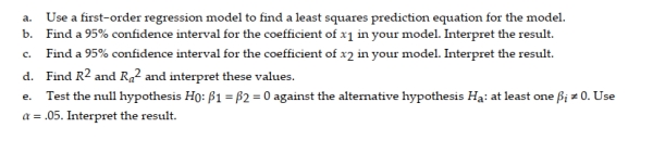
As part of a study at a large university, data were collected on n = 224 freshmen computer science (CS) majors in a particular year. The researchers were interested in modeling y, a student's grade point average (GPA) after three semesters, as a function of the following independent variables (recorded at the time the students enrolled in the university): 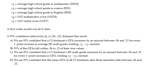
Question
Question
Question
Question
Question
Retail price data for n = 60 hard disk drives were recently reported in a computer magazine. Three variables were recorded for each hard disk drive: 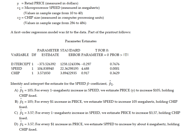
Question
Retail price data for n = 60 hard disk drives were recently reported in a computer magazine. Three variables were recorded for each hard disk drive: 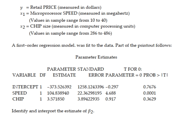
Question
Question
Question
Question
The printout shows the results of a first-order regression analysis relating the sales price y of a product to the time in hours x1 and the cost of raw materials x2 needed to make the product. 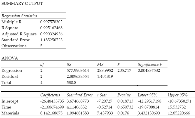 a. What is the least squares prediction equation? b. Identify the SSE from the printout. c. Find the estimator of σ2 for the model.
a. What is the least squares prediction equation? b. Identify the SSE from the printout. c. Find the estimator of σ2 for the model. Question
Question
Question
A statistics professor gave three quizzes leading up to the first test in his class. The quiz grades and test grade for each of eight students are given in the table. 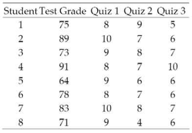 The professor would like to use the data to find a first-order model that he might use to predict a student's grade on the first test using that student's grades on the first three quizzes. a. Identify the dependent and independent variables for the model. b. What is the least squares prediction equation? c. Find the SSE and the estimator of σ2 for the model. 2 Find and Interpret Sample Estimates for β Parameters
The professor would like to use the data to find a first-order model that he might use to predict a student's grade on the first test using that student's grades on the first three quizzes. a. Identify the dependent and independent variables for the model. b. What is the least squares prediction equation? c. Find the SSE and the estimator of σ2 for the model. 2 Find and Interpret Sample Estimates for β Parameters Question
Question
Retail price data for n = 60 hard disk drives were recently reported in a computer magazine. Three variables were recorded for each hard disk drive: 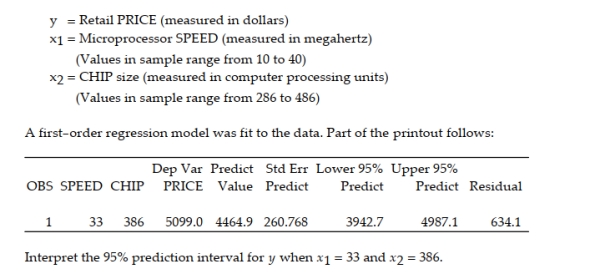 2 Find and Interpret Confidence Interval
2 Find and Interpret Confidence Interval Question
A study of the top MBA programs attempted to predict the average starting salary (in $1000's) of graduates of the program based on the amount of tuition (in $1000's) charged by the program and the average GMAT score of the program's students. The results of a regression analysis based on a sample of 75 MBA programs is shown below: Least Squares Linear Regression of Salary 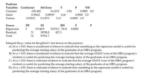
Question
A study of the top MBA programs attempted to predict the average starting salary (in $1000's) of graduates of the program based on the amount of tuition (in $1000's) charged by the program and the average GMAT score of the program's students. The results of a regression analysis based on a sample of 75 MBA programs is shown below: Least Squares Linear Regression of Salary 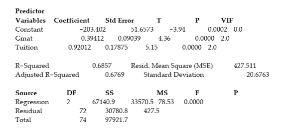 Interpret the coefficient of determination value shown in the printout.
A) We can explain 68.57% of the variation in the average starting salaries around their mean using the model that includes the average GMAT score and the tuition for the MBA program.
B) We expect most of the average starting salaries to fall within $41,353 of their least squares predicted values.
C) We expect most of the average starting salaries to fall within $20,676 of their least squares predicted values.
D) At α = 0.05, there is insufficient evidence to indicate that something in the regression model is useful for predicting the average starting salary of the graduates of an MBA program.
Interpret the coefficient of determination value shown in the printout.A) We can explain 68.57% of the variation in the average starting salaries around their mean using the model that includes the average GMAT score and the tuition for the MBA program.
B) We expect most of the average starting salaries to fall within $41,353 of their least squares predicted values.
C) We expect most of the average starting salaries to fall within $20,676 of their least squares predicted values.
D) At α = 0.05, there is insufficient evidence to indicate that something in the regression model is useful for predicting the average starting salary of the graduates of an MBA program.
Question
A statistics professor gave three quizzes leading up to the first test in his class. The quiz grades and test grade for each of eight students are given in the table. 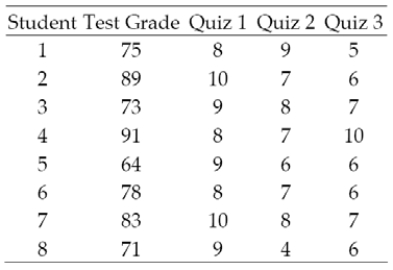 The professor fit a first-order model to the data that he intends to use to predict a student's grade on the first test using that student's grades on the first three quizzes.
  α = .05. Interpret the result. 12.4 Using the Model for Estimation and Prediction 1 Find and Interpret Prediction Interval
The professor fit a first-order model to the data that he intends to use to predict a student's grade on the first test using that student's grades on the first three quizzes. α = .05. Interpret the result. 12.4 Using the Model for Estimation and Prediction 1 Find and Interpret Prediction Interval Question
Question
As part of a study at a large university, data were collected on n = 224 freshmen computer science (CS) majors in a particular year. The researchers were interested in modeling y, a student's grade point average (GPA) after three semesters, as a function of the following independent variables (recorded at the time the students enrolled in the university): 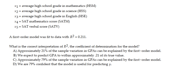
Question
Question
The table below shows data for n = 20 observations. 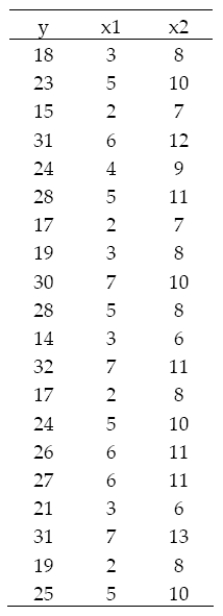
Question
As part of a study at a large university, data were collected on n = 224 freshmen computer science (CS) majors in a particular year. The researchers were interested in modeling y, a student's grade point average (GPA) after three semesters, as a function of the following independent variables (recorded at the time the students enrolled in the university): 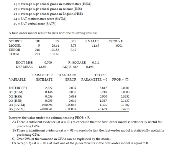
Question
A study of the top MBA programs attempted to predict the average starting salary (in $1000's) of graduates of the program based on the amount of tuition (in $1000's) charged by the program and the average GMAT score of the program's students. The results of a regression analysis based on a sample of 75 MBA programs is shown below: Least Squares Linear Regression of Salary 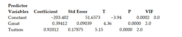 The model was then used to create 95% confidence and prediction intervals for y and for E(Y) when the tuition charged by the MBA program was $75,000 and the GMAT score was 675. The results are shown here: 95% confidence interval for E(Y): ($126,610, $136,640) 95% prediction interval for Y: ($90,113, $173,160) Which of the following interpretations is correct if you want to use the model to estimate Y for a single MBA program?
A) We are 95% confident that the average starting salary for graduates of a single MBA program that charges $75,000 in tuition and has an average GMAT score of 675 will fall between $126,610 and $136,640.
B) We are 95% confident that the average starting salary for graduates of a single MBA program that charges $75,000 in tuition and has an average GMAT score of 675 will fall between $90,113 and $173,16,30.
C) We are 95% confident that the average of all starting salaries for graduates of all MBA programs that charge $75,000 in tuition and have an average GMAT score of 675 will fall between $126,610 and $136,640.
D) We are 95% confident that the average of all starting salaries for graduates of all MBA programs that charge $75,000 in tuition and have an average GMAT score of 675 will fall between $90,113 and
$173,16,30.
The model was then used to create 95% confidence and prediction intervals for y and for E(Y) when the tuition charged by the MBA program was $75,000 and the GMAT score was 675. The results are shown here: 95% confidence interval for E(Y): ($126,610, $136,640) 95% prediction interval for Y: ($90,113, $173,160) Which of the following interpretations is correct if you want to use the model to estimate Y for a single MBA program?A) We are 95% confident that the average starting salary for graduates of a single MBA program that charges $75,000 in tuition and has an average GMAT score of 675 will fall between $126,610 and $136,640.
B) We are 95% confident that the average starting salary for graduates of a single MBA program that charges $75,000 in tuition and has an average GMAT score of 675 will fall between $90,113 and $173,16,30.
C) We are 95% confident that the average of all starting salaries for graduates of all MBA programs that charge $75,000 in tuition and have an average GMAT score of 675 will fall between $126,610 and $136,640.
D) We are 95% confident that the average of all starting salaries for graduates of all MBA programs that charge $75,000 in tuition and have an average GMAT score of 675 will fall between $90,113 and
$173,16,30.
Question
As part of a study at a large university, data were collected on n = 224 freshmen computer science (CS) majors in a particular year. The researchers were interested in modeling y, a student's grade point average (GPA) after three semesters, as a function of the following independent variables (recorded at the time the students enrolled in the university): 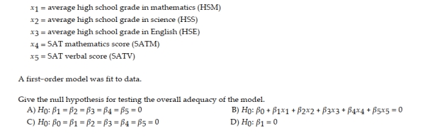
Question
As part of a study at a large university, data were collected on n = 224 freshmen computer science (CS) majors in a particular year. The researchers were interested in modeling y, a student's grade point average (GPA) after three semesters, as a function of the following independent variables (recorded at the time the students enrolled in the university): 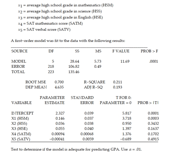
Question
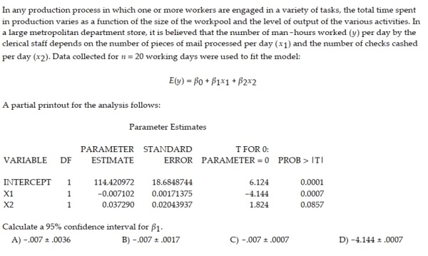
In any production process in which one or more workers are engaged in a variety of tasks, the total time spent in production varies as a function of the size of the workpool and the level of output of the various activities. In a large metropolitan department store, it is believed that the number of man-hours worked (y) per day by the clerical staff depends on the number of pieces of mail processed per day (x1) and the number of checks cashed per day (x2). Data collected for n = 20 working days were used to fit the model: 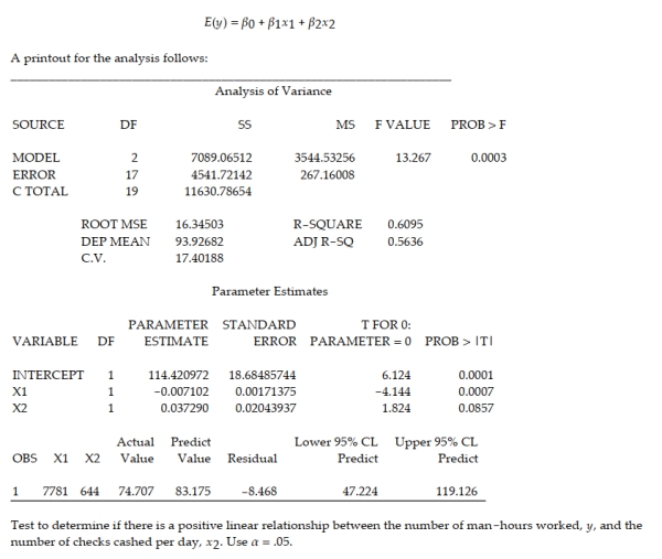
Question
Retail price data for n = 60 hard disk drives were recently reported in a computer magazine. Three variables were recorded for each hard disk drive: 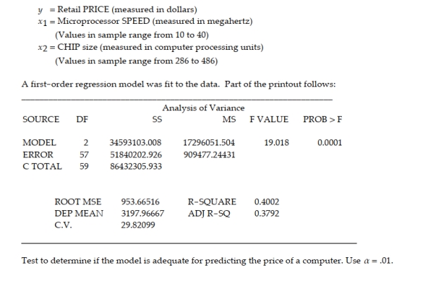
Question
In any production process in which one or more workers are engaged in a variety of tasks, the total time spent in production varies as a function of the size of the workpool and the level of output of the various activities. In a large metropolitan department store, it is believed that the number of man-hours worked (y) per day by the clerical staff depends on the number of pieces of mail processed per day (x1) and the number of checks cashed per day (x2). Data collected for n = 20 working days were used to fit the model: 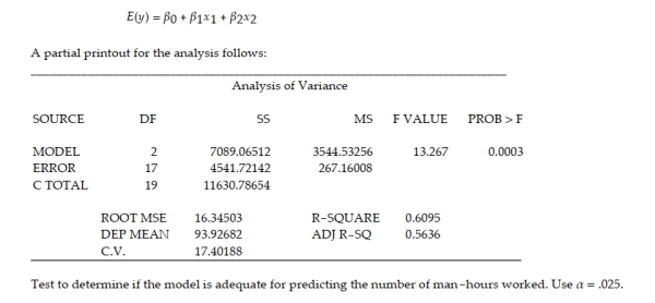
Question
Question
Question
As part of a study at a large university, data were collected on n = 224 freshmen computer science (CS) majors in a particular year. The researchers were interested in modeling y, a student's grade point average (GPA) after three semesters, as a function of the following independent variables (recorded at the time the students enrolled in the university): 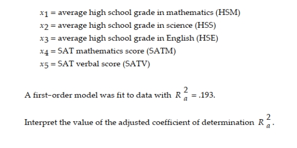
Question
Question
Question
A college admissions officer proposes to use regression to model a student's college GPA at graduation in terms of the following two variables: 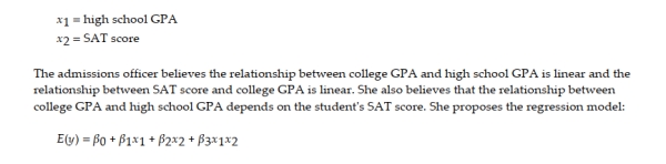 Explain how to determine if the relationship between college GPA and SAT score depends on the high school GPA.
Explain how to determine if the relationship between college GPA and SAT score depends on the high school GPA. Question
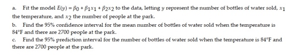
The concessions manager at a beachside park recorded the high temperature, the number of people at the park, and the number of bottles of water sold for each of 12 consecutive Saturdays. The data are shown below. 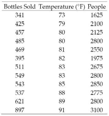
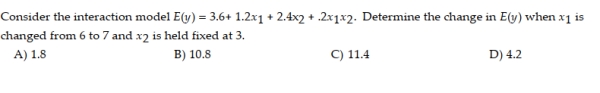
 12.5 Interaction Models 1 Write Interaction Model
12.5 Interaction Models 1 Write Interaction Model Question
Question
Question
A study of the top MBA programs attempted to predict the average starting salary (in $1000's) of graduates of the program based on the amount of tuition (in $1000's) charged by the program and the average GMAT score of the program's students. The results of a regression analysis based on a sample of 75 MBA programs is shown below: Least Squares Linear Regression of Salary 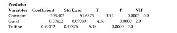 The model was then used to create 95% confidence and prediction intervals for y and for E(Y) when the tuition charged by the MBA program was $75,000 and the GMAT score was 675. The results are shown here: 95% confidence interval for E(Y): ($126,610, $136,640) 95% prediction interval for Y: ($90,113, $173,160) Which of the following interpretations is correct if you want to use the model to estimate E(Y) for all MBA programs?
A) We are 95% confident that the average starting salary for graduates of a single MBA program that charges $75,000 in tuition and has an average GMAT score of 675 will fall between $126,610 and $136,640.
B) We are 95% confident that the average starting salary for graduates of a single MBA program that charges $75,000 in tuition and has an average GMAT score of 675 will fall between $90,113 and $173,16,30.
C) We are 95% confident that the average of all starting salaries for graduates of all MBA programs that charge $75,000 in tuition and have an average GMAT score of 675 will fall between $126,610 and $136,640.
D) We are 95% confident that the average of all starting salaries for graduates of all MBA programs that charge $75,000 in tuition and have an average GMAT score of 675 will fall between $90,113 and
$173,16,30.
The model was then used to create 95% confidence and prediction intervals for y and for E(Y) when the tuition charged by the MBA program was $75,000 and the GMAT score was 675. The results are shown here: 95% confidence interval for E(Y): ($126,610, $136,640) 95% prediction interval for Y: ($90,113, $173,160) Which of the following interpretations is correct if you want to use the model to estimate E(Y) for all MBA programs?A) We are 95% confident that the average starting salary for graduates of a single MBA program that charges $75,000 in tuition and has an average GMAT score of 675 will fall between $126,610 and $136,640.
B) We are 95% confident that the average starting salary for graduates of a single MBA program that charges $75,000 in tuition and has an average GMAT score of 675 will fall between $90,113 and $173,16,30.
C) We are 95% confident that the average of all starting salaries for graduates of all MBA programs that charge $75,000 in tuition and have an average GMAT score of 675 will fall between $126,610 and $136,640.
D) We are 95% confident that the average of all starting salaries for graduates of all MBA programs that charge $75,000 in tuition and have an average GMAT score of 675 will fall between $90,113 and
$173,16,30.
Question
Question
Question
Question
Question
A collector of grandfather clocks believes that the price received for the clocks at an auction increases with the number of bidders, but at an increasing (rather than a constant) rate. Thus, the model proposed to best explain auction price (y, in dollars) by number of bidders (x) is the quadratic model 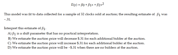
Question
A college admissions officer proposes to use regression to model a student's college GPA at graduation in terms of the following two variables: 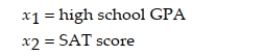 The admissions officer believes the relationship between college GPA and high school GPA is linear and the relationship between SAT score and college GPA is linear. She also believes that the relationship between college GPA and high school GPA depends on the student's SAT score. Write the regression model she should fit. 2 Test if Model is Useful for Predicting y
The admissions officer believes the relationship between college GPA and high school GPA is linear and the relationship between SAT score and college GPA is linear. She also believes that the relationship between college GPA and high school GPA depends on the student's SAT score. Write the regression model she should fit. 2 Test if Model is Useful for Predicting y Question
Which equation represents a complete second-order model for two quantitative independent variables? 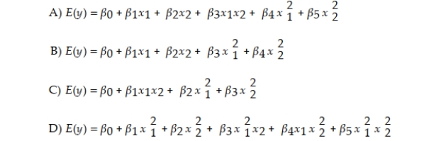
Question
Question
A study of the top MBA programs attempted to predict the average starting salary (in $1000's) of graduates of the program based on the amount of tuition (in $1000's) charged by the program and the average GMAT score of the program's students. The results of a regression analysis based on a sample of 75 MBA programs is shown below: Least Squares Linear Regression of Salary 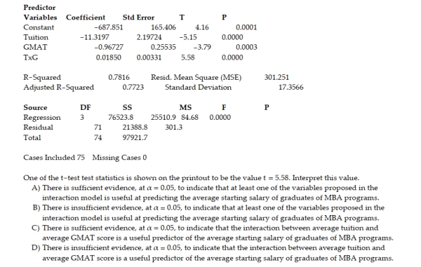
Question
Consider the partial printout below. 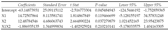 Is there evidence (at α = .05) that x1 and x2 interact? Explain. 12.6 Quadratic and Other Higher Order Models 1 Write and Interpret Second-Order Model
Is there evidence (at α = .05) that x1 and x2 interact? Explain. 12.6 Quadratic and Other Higher Order Models 1 Write and Interpret Second-Order Model Question
A study of the top MBA programs attempted to predict the average starting salary (in $1000's) of graduates of the program based on the amount of tuition (in $1000's) charged by the program and the average GMAT score of the program's students. The results of a regression analysis based on a sample of 75 MBA programs is shown below: Least Squares Linear Regression of Salary 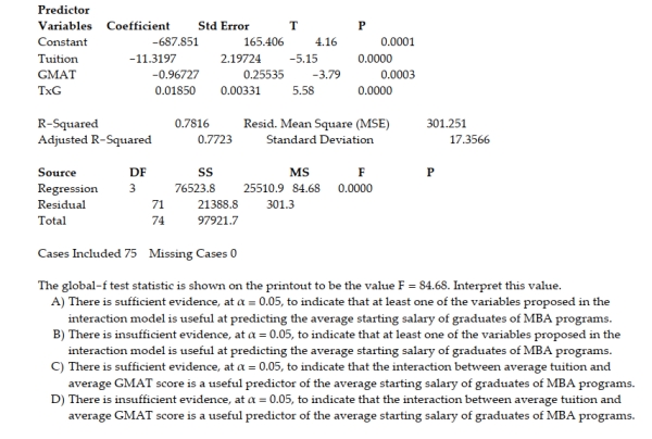
Question
Question
Consider the partial printout for an interaction regression analysis of the relationship between a dependent variable y and two independent variables x1 and x2. 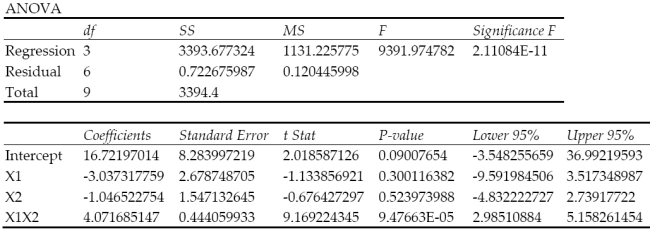
 3 Test for Interaction Between Two Variables
3 Test for Interaction Between Two Variables Question
Question
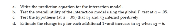
A certain type of rare gem serves as a status symbol for many of its owners. In theory, for low prices, the demand decreases as the price of the gem increases. However, experts hypothesize that when the gem is valued at very high prices, the demand increases with price due to the status the owners believe they gain by obtaining the gem. Thus, the model proposed to best explain the demand for the gem by its price is the quadratic model 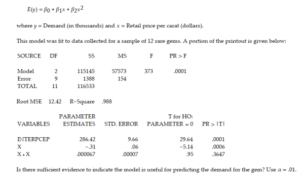
Question
Question
Question
A certain type of rare gem serves as a status symbol for many of its owners. In theory, for low prices, the demand decreases as the price of the gem increases. However, experts hypothesize that when the gem is valued at very high prices, the demand increases with price due to the status the owners believe they gain by obtaining the gem. Thus, the model proposed to best explain the demand for the gem by its price is the quadratic model 
Question
Question
The complete second-order model  data points. The printout is shown below.
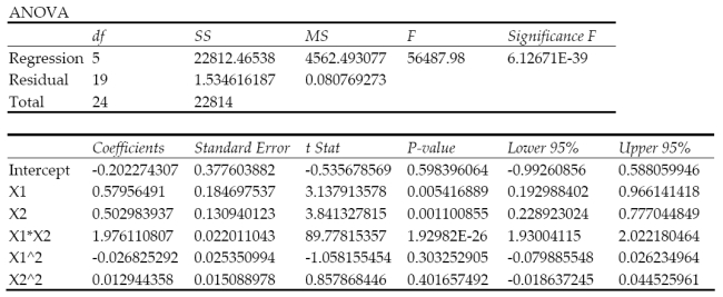
 3 Test if Model is Useful for Predicting y
data points. The printout is shown below. 3 Test if Model is Useful for Predicting y Question
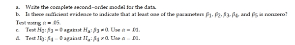
A study of the top MBA programs attempted to predict y = the average starting salary (in $1000's) of graduates of the program based on x = the amount of tuition (in $1000's) charged by the program. After first considering a simple linear model, it was decided that a quadratic model should be proposed. Which of the following models proposes a 2nd-order quadratic relationship between x and y? 
Question
What relationship between x and y is suggested by the scattergram? 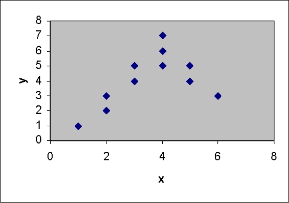
A) a quadratic relationship with downward concavity
B) a quadratic relationship with upward concavity
C) a linear relationship with positive slope
D) a linear relationship with negative slope
A) a quadratic relationship with downward concavity
B) a quadratic relationship with upward concavity
C) a linear relationship with positive slope
D) a linear relationship with negative slope
Question
A study of the top MBA programs attempted to predict the average starting salary (in $1000's) of graduates of the program based on the amount of tuition (in $1000's) charged by the program and the average GMAT score of the program's students. The results of a regression analysis based on a sample of 75 MBA programs is shown below: Least Squares Linear Regression of Salary 
Question
Question
Consider the second-order model 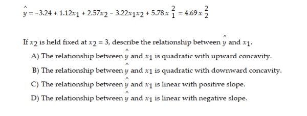
Question
The table shows the profit y (in thousands of dollars) that a company made during a month when the price of its product was x dollars per unit. 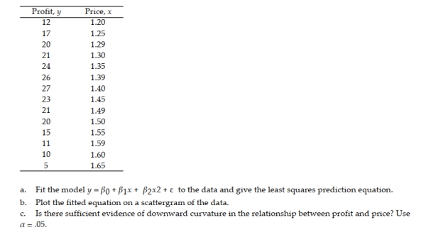 4 Perform Quadratic Regression and Make Predictions
4 Perform Quadratic Regression and Make Predictions Question
A study of the top MBA programs attempted to predict the average starting salary (in $1000's) of graduates of the program based on the amount of tuition (in $1000's) charged by the program and the average GMAT score of the program's students. The results of a regression analysis based on a sample of 75 MBA programs is shown below: Least Squares Linear Regression of Salary 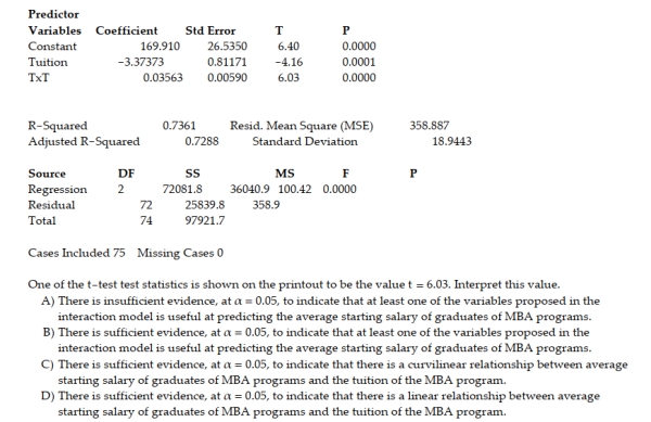
Question
Question
A graphing calculator was used to fit the model E(y) = ?0 + ?1x + ?2x2 to a set of data. The resulting screen is shown below. 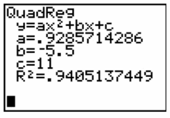 Which number on the screen represents the estimator of ?
A) .9286
B) 5.5
C) 11
D) .9405
Which number on the screen represents the estimator of ?A) .9286
B) 5.5
C) 11
D) .9405
Question
A certain type of rare gem serves as a status symbol for many of its owners. In theory, for low prices, the demand decreases as the price of the gem increases. However, experts hypothesize that when the gem is valued at very high prices, the demand increases with price due to the status the owners believe they gain by obtaining the gem. Thus, the model proposed to best explain the demand for the gem by its price is the quadratic model 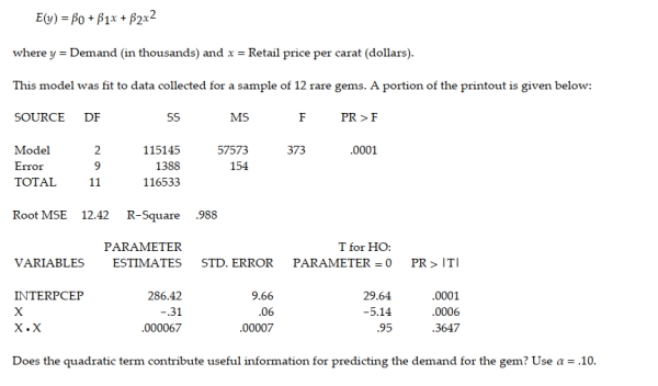
Question
Consider the data given in the table below. 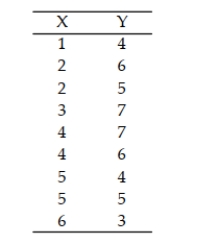 a. Plot the data on a scattergram. Does a quadratic model seem to be a good fit for the data? Explain. b. Use the method of least squares to find a quadratic prediction equation. c. Graph the prediction equation on your scattergram. 12.7 Qualitative (Dummy) Variable Models 1 Write and Interpret Model with Qualitative Variables
a. Plot the data on a scattergram. Does a quadratic model seem to be a good fit for the data? Explain. b. Use the method of least squares to find a quadratic prediction equation. c. Graph the prediction equation on your scattergram. 12.7 Qualitative (Dummy) Variable Models 1 Write and Interpret Model with Qualitative Variables Question
Consider the data given in the table below. 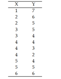 Plot the data on a scattergram. Does a second-order model seem to be a good fit for the data? Explain.
Plot the data on a scattergram. Does a second-order model seem to be a good fit for the data? Explain. Question
A collector of grandfather clocks believes that the price received for the clocks at an auction increases with the number of bidders, but at an increasing (rather than a constant) rate. Thus, the model proposed to best explain auction price (y, in dollars) by number of bidders (x) is the quadratic model 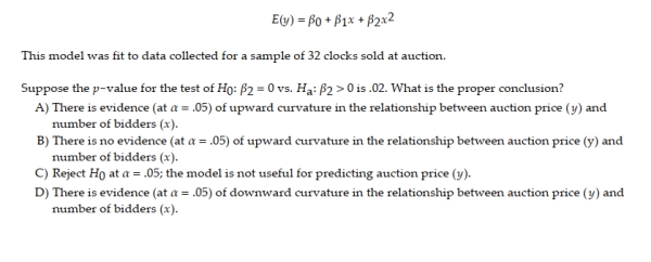
Question
A certain type of rare gem serves as a status symbol for many of its owners. In theory, for low prices, the demand decreases as the price of the gem increases. However, experts hypothesize that when the gem is valued at very high prices, the demand increases with price due to the status the owners believe they gain by obtaining the gem. Thus, the model proposed to best explain the demand for the gem by its price is the quadratic model 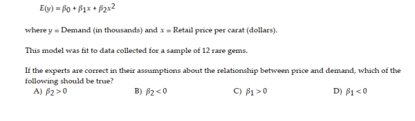

Unlock Deck
Sign up to unlock the cards in this deck!
Unlock Deck
Unlock Deck
1/131
Play
Full screen (f)
Deck 12: Multiple Regression and Model Building
1
It is safe to conduct t-tests on the individual β parameters in a first-order linear model in order to determine which independent variables are useful for predicting y and which are not.
False
2
A qualitative variable whose outcomes are assigned numerical values is called a coded variable.
True
3
A study of the top MBA programs attempted to predict the average starting salary (in $1000's) of graduates of the program based on the amount of tuition (in $1000's) charged by the program and the average GMAT score of the program's students. The results of a regression analysis based on a sample of 75 MBA programs is shown below: Least Squares Linear Regression of Salary
C
4
Unlock Deck
Unlock for access to all 131 flashcards in this deck.
Unlock Deck
k this deck
5
A study of the top MBA programs attempted to predict the average starting salary (in $1000's) of graduates of the program based on the amount of tuition (in $1000's) charged by the program and the average GMAT score of the program's students. The results of a regression analysis based on a sample of 75 MBA programs is shown below: Least Squares Linear Regression of Salary Interpret the coefficient for the tuition variable shown on the printout.
A) For every $1000 increase in the tuition charged by the MBA program, we estimate that the average starting salary will decrease by $203,402, holding the GMAT score constant.
B) For every $1000 increase in the tuition charged by the MBA program, we estimate that the average starting salary will increase by $394.12, holding the GMAT score constant
C) For every $1000 increase in the tuition charged by the MBA program, we estimate that the average starting salary will increase by $920.12, holding the GMAT score constant
D) For every $1000 increase in the average starting salary, we estimate that the tuition charged by the MBA program will increase by $920.12.
Interpret the coefficient for the tuition variable shown on the printout.A) For every $1000 increase in the tuition charged by the MBA program, we estimate that the average starting salary will decrease by $203,402, holding the GMAT score constant.
B) For every $1000 increase in the tuition charged by the MBA program, we estimate that the average starting salary will increase by $394.12, holding the GMAT score constant
C) For every $1000 increase in the tuition charged by the MBA program, we estimate that the average starting salary will increase by $920.12, holding the GMAT score constant
D) For every $1000 increase in the average starting salary, we estimate that the tuition charged by the MBA program will increase by $920.12.
Unlock Deck
Unlock for access to all 131 flashcards in this deck.
Unlock Deck
k this deck
6
Why is the random error term ε added to a multiple regression model? 12.2 Estimating and Making Inferences about the β Parameters 1 Write First-Order Model
Unlock Deck
Unlock for access to all 131 flashcards in this deck.
Unlock Deck
k this deck
7
As part of a study at a large university, data were collected on n = 224 freshmen computer science (CS) majors in a particular year. The researchers were interested in modeling y, a student's grade point average (GPA) after three semesters, as a function of the following independent variables (recorded at the time the students enrolled in the university):
Unlock Deck
Unlock for access to all 131 flashcards in this deck.
Unlock Deck
k this deck
8
For a multiple regression model, we assume that the mean of the probability distribution of the random error is 0.
Unlock Deck
Unlock for access to all 131 flashcards in this deck.
Unlock Deck
k this deck
9
Unlock Deck
Unlock for access to all 131 flashcards in this deck.
Unlock Deck
k this deck
10
Unlock Deck
Unlock for access to all 131 flashcards in this deck.
Unlock Deck
k this deck
11
In the first-order model represents the slope of the line relating to when and are both held fixed.
Unlock Deck
Unlock for access to all 131 flashcards in this deck.
Unlock Deck
k this deck
12
Retail price data for n = 60 hard disk drives were recently reported in a computer magazine. Three variables were recorded for each hard disk drive:
Unlock Deck
Unlock for access to all 131 flashcards in this deck.
Unlock Deck
k this deck
13
Retail price data for n = 60 hard disk drives were recently reported in a computer magazine. Three variables were recorded for each hard disk drive:
Unlock Deck
Unlock for access to all 131 flashcards in this deck.
Unlock Deck
k this deck
14
A first-order model does not contain any higher-order terms.
Unlock Deck
Unlock for access to all 131 flashcards in this deck.
Unlock Deck
k this deck
15
A first-order model may include terms for both quantitative and qualitative independent variables.
Unlock Deck
Unlock for access to all 131 flashcards in this deck.
Unlock Deck
k this deck
16
The method of fitting first-order models is the same as that of fitting the simple straight-line model, i.e. the method of least squares.
Unlock Deck
Unlock for access to all 131 flashcards in this deck.
Unlock Deck
k this deck
17
The printout shows the results of a first-order regression analysis relating the sales price y of a product to the time in hours x1 and the cost of raw materials x2 needed to make the product. a. What is the least squares prediction equation? b. Identify the SSE from the printout. c. Find the estimator of σ2 for the model.
a. What is the least squares prediction equation? b. Identify the SSE from the printout. c. Find the estimator of σ2 for the model. Unlock Deck
Unlock for access to all 131 flashcards in this deck.
Unlock Deck
k this deck
18
A term that contains the value of a quantitative variable raised to the second power is called a higher -order term.
Unlock Deck
Unlock for access to all 131 flashcards in this deck.
Unlock Deck
k this deck
19
Probabilistic models that include more than one dependent variable are called multiple regression models.
Unlock Deck
Unlock for access to all 131 flashcards in this deck.
Unlock Deck
k this deck
20
A statistics professor gave three quizzes leading up to the first test in his class. The quiz grades and test grade for each of eight students are given in the table. The professor would like to use the data to find a first-order model that he might use to predict a student's grade on the first test using that student's grades on the first three quizzes. a. Identify the dependent and independent variables for the model. b. What is the least squares prediction equation? c. Find the SSE and the estimator of σ2 for the model. 2 Find and Interpret Sample Estimates for β Parameters
The professor would like to use the data to find a first-order model that he might use to predict a student's grade on the first test using that student's grades on the first three quizzes. a. Identify the dependent and independent variables for the model. b. What is the least squares prediction equation? c. Find the SSE and the estimator of σ2 for the model. 2 Find and Interpret Sample Estimates for β Parameters Unlock Deck
Unlock for access to all 131 flashcards in this deck.
Unlock Deck
k this deck
21
The value of R2 is only useful when the number of data points is substantially larger than the number of β parameters in the model.
Unlock Deck
Unlock for access to all 131 flashcards in this deck.
Unlock Deck
k this deck
22
Retail price data for n = 60 hard disk drives were recently reported in a computer magazine. Three variables were recorded for each hard disk drive: 2 Find and Interpret Confidence Interval
2 Find and Interpret Confidence Interval Unlock Deck
Unlock for access to all 131 flashcards in this deck.
Unlock Deck
k this deck
23
A study of the top MBA programs attempted to predict the average starting salary (in $1000's) of graduates of the program based on the amount of tuition (in $1000's) charged by the program and the average GMAT score of the program's students. The results of a regression analysis based on a sample of 75 MBA programs is shown below: Least Squares Linear Regression of Salary
Unlock Deck
Unlock for access to all 131 flashcards in this deck.
Unlock Deck
k this deck
24
A study of the top MBA programs attempted to predict the average starting salary (in $1000's) of graduates of the program based on the amount of tuition (in $1000's) charged by the program and the average GMAT score of the program's students. The results of a regression analysis based on a sample of 75 MBA programs is shown below: Least Squares Linear Regression of Salary Interpret the coefficient of determination value shown in the printout.
A) We can explain 68.57% of the variation in the average starting salaries around their mean using the model that includes the average GMAT score and the tuition for the MBA program.
B) We expect most of the average starting salaries to fall within $41,353 of their least squares predicted values.
C) We expect most of the average starting salaries to fall within $20,676 of their least squares predicted values.
D) At α = 0.05, there is insufficient evidence to indicate that something in the regression model is useful for predicting the average starting salary of the graduates of an MBA program.
Interpret the coefficient of determination value shown in the printout.A) We can explain 68.57% of the variation in the average starting salaries around their mean using the model that includes the average GMAT score and the tuition for the MBA program.
B) We expect most of the average starting salaries to fall within $41,353 of their least squares predicted values.
C) We expect most of the average starting salaries to fall within $20,676 of their least squares predicted values.
D) At α = 0.05, there is insufficient evidence to indicate that something in the regression model is useful for predicting the average starting salary of the graduates of an MBA program.
Unlock Deck
Unlock for access to all 131 flashcards in this deck.
Unlock Deck
k this deck
25
A statistics professor gave three quizzes leading up to the first test in his class. The quiz grades and test grade for each of eight students are given in the table. The professor fit a first-order model to the data that he intends to use to predict a student's grade on the first test using that student's grades on the first three quizzes. α = .05. Interpret the result. 12.4 Using the Model for Estimation and Prediction 1 Find and Interpret Prediction Interval
The professor fit a first-order model to the data that he intends to use to predict a student's grade on the first test using that student's grades on the first three quizzes. α = .05. Interpret the result. 12.4 Using the Model for Estimation and Prediction 1 Find and Interpret Prediction Interval Unlock Deck
Unlock for access to all 131 flashcards in this deck.
Unlock Deck
k this deck
26
In any production process in which one or more workers are engaged in a variety of tasks, the total time spent in production varies as a function of the size of the workpool and the level of output of the various activities. In a large metropolitan department store, it is believed that the number of man-hours worked (y) per day by the clerical staff depends on the number of pieces of mail processed per day (x1) and the number of checks cashed per day (x2). Data collected for n = 20 working days were used to fit the model:
A partial printout for the analysis follows:
Interpret the 95% prediction interval for y shown on the printout.
A) We are 95% confident that between 47.224 and 119.126 man-hours will be worked during a single day in which 7,781 pieces of mail are processed and 644 checks are cashed.
B) We expect to predict number of man-hours worked per day to within an amount between 47.224 and 119.126 of the true value.
C) We are 95% confident that the number of man-hours worked per day falls between 47.224 and 119.126.
D) We are 95% confident that the mean number of man-hours worked per day falls between 47.224 and 119.126 for all days in which 7,781 pieces of mail are processed and 644 checks are cashed.
Unlock Deck
Unlock for access to all 131 flashcards in this deck.
Unlock Deck
k this deck
27
As part of a study at a large university, data were collected on n = 224 freshmen computer science (CS) majors in a particular year. The researchers were interested in modeling y, a student's grade point average (GPA) after three semesters, as a function of the following independent variables (recorded at the time the students enrolled in the university):
Unlock Deck
Unlock for access to all 131 flashcards in this deck.
Unlock Deck
k this deck
28
The confidence interval for the mean E(y) is narrower that the prediction interval for y.
Unlock Deck
Unlock for access to all 131 flashcards in this deck.
Unlock Deck
k this deck
29
The table below shows data for n = 20 observations.
Unlock Deck
Unlock for access to all 131 flashcards in this deck.
Unlock Deck
k this deck
30
As part of a study at a large university, data were collected on n = 224 freshmen computer science (CS) majors in a particular year. The researchers were interested in modeling y, a student's grade point average (GPA) after three semesters, as a function of the following independent variables (recorded at the time the students enrolled in the university):
Unlock Deck
Unlock for access to all 131 flashcards in this deck.
Unlock Deck
k this deck
31
A study of the top MBA programs attempted to predict the average starting salary (in $1000's) of graduates of the program based on the amount of tuition (in $1000's) charged by the program and the average GMAT score of the program's students. The results of a regression analysis based on a sample of 75 MBA programs is shown below: Least Squares Linear Regression of Salary The model was then used to create 95% confidence and prediction intervals for y and for E(Y) when the tuition charged by the MBA program was $75,000 and the GMAT score was 675. The results are shown here: 95% confidence interval for E(Y): ($126,610, $136,640) 95% prediction interval for Y: ($90,113, $173,160) Which of the following interpretations is correct if you want to use the model to estimate Y for a single MBA program?
A) We are 95% confident that the average starting salary for graduates of a single MBA program that charges $75,000 in tuition and has an average GMAT score of 675 will fall between $126,610 and $136,640.
B) We are 95% confident that the average starting salary for graduates of a single MBA program that charges $75,000 in tuition and has an average GMAT score of 675 will fall between $90,113 and $173,16,30.
C) We are 95% confident that the average of all starting salaries for graduates of all MBA programs that charge $75,000 in tuition and have an average GMAT score of 675 will fall between $126,610 and $136,640.
D) We are 95% confident that the average of all starting salaries for graduates of all MBA programs that charge $75,000 in tuition and have an average GMAT score of 675 will fall between $90,113 and
$173,16,30.
The model was then used to create 95% confidence and prediction intervals for y and for E(Y) when the tuition charged by the MBA program was $75,000 and the GMAT score was 675. The results are shown here: 95% confidence interval for E(Y): ($126,610, $136,640) 95% prediction interval for Y: ($90,113, $173,160) Which of the following interpretations is correct if you want to use the model to estimate Y for a single MBA program?A) We are 95% confident that the average starting salary for graduates of a single MBA program that charges $75,000 in tuition and has an average GMAT score of 675 will fall between $126,610 and $136,640.
B) We are 95% confident that the average starting salary for graduates of a single MBA program that charges $75,000 in tuition and has an average GMAT score of 675 will fall between $90,113 and $173,16,30.
C) We are 95% confident that the average of all starting salaries for graduates of all MBA programs that charge $75,000 in tuition and have an average GMAT score of 675 will fall between $126,610 and $136,640.
D) We are 95% confident that the average of all starting salaries for graduates of all MBA programs that charge $75,000 in tuition and have an average GMAT score of 675 will fall between $90,113 and
$173,16,30.
Unlock Deck
Unlock for access to all 131 flashcards in this deck.
Unlock Deck
k this deck
32
As part of a study at a large university, data were collected on n = 224 freshmen computer science (CS) majors in a particular year. The researchers were interested in modeling y, a student's grade point average (GPA) after three semesters, as a function of the following independent variables (recorded at the time the students enrolled in the university):
Unlock Deck
Unlock for access to all 131 flashcards in this deck.
Unlock Deck
k this deck
33
As part of a study at a large university, data were collected on n = 224 freshmen computer science (CS) majors in a particular year. The researchers were interested in modeling y, a student's grade point average (GPA) after three semesters, as a function of the following independent variables (recorded at the time the students enrolled in the university):
Unlock Deck
Unlock for access to all 131 flashcards in this deck.
Unlock Deck
k this deck
34
In any production process in which one or more workers are engaged in a variety of tasks, the total time spent in production varies as a function of the size of the workpool and the level of output of the various activities. In a large metropolitan department store, it is believed that the number of man-hours worked (y) per day by the clerical staff depends on the number of pieces of mail processed per day (x1) and the number of checks cashed per day (x2). Data collected for n = 20 working days were used to fit the model:
Unlock Deck
Unlock for access to all 131 flashcards in this deck.
Unlock Deck
k this deck
35
Retail price data for n = 60 hard disk drives were recently reported in a computer magazine. Three variables were recorded for each hard disk drive:
Unlock Deck
Unlock for access to all 131 flashcards in this deck.
Unlock Deck
k this deck
36
In any production process in which one or more workers are engaged in a variety of tasks, the total time spent in production varies as a function of the size of the workpool and the level of output of the various activities. In a large metropolitan department store, it is believed that the number of man-hours worked (y) per day by the clerical staff depends on the number of pieces of mail processed per day (x1) and the number of checks cashed per day (x2). Data collected for n = 20 working days were used to fit the model:
Unlock Deck
Unlock for access to all 131 flashcards in this deck.
Unlock Deck
k this deck
37
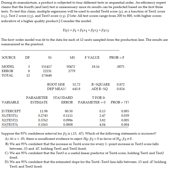
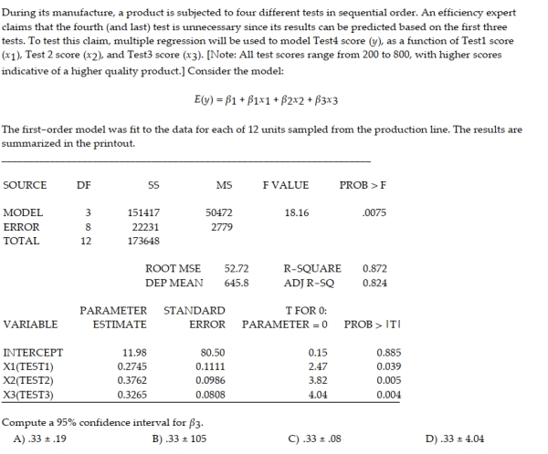
During its manufacture, a product is subjected to four different tests in sequential order. An efficiency expert claims that the fourth (and last) test is unnecessary since its results can be predicted based on the first three tests. To test this claim, multiple regression will be used to model Test 4 score (y), as a function of Test1 score , Test 2 score , and Test3 score . [Note: All test scores range from 200 to 800 , with higher scores indicative of a higher quality product.] Consider the model:
The global statistic is used to test the null hypothesis, . Describe this hypothesis in words.
A) The model is not statistically useful for predicting Test4 score.
B) The model is statistically useful for predicting Test4 score.
C) The first three test scores are poor predictors of Test4 score.
D) The first three test scores are reliable predictors of Test4 score.
Unlock Deck
Unlock for access to all 131 flashcards in this deck.
Unlock Deck
k this deck
38
During its manufacture, a product is subjected to four different tests in sequential order. An efficiency expert claims that the fourth (and last) test is unnecessary since its results can be predicted based on the first three tests. To test this claim, multiple regression will be used to model Test4 score (y), as a function of Test1 score (x1), Test 2 score (x2), and Test3 score (x3). [Note: All test scores range from 200 to 800, with higher scores indicative of a higher quality product.] Consider the model: The first-order model was fit to the data for each of 12 units sampled from the production line. A 95% prediction interval for Test4 score of a product with Test1 = 590, Test2 = 750, and Test3 = 710 is (583, 793). Interpret this result.
A) We are 95% confident that a product's Test4 score will fall between 583 and 793 points when the first three scores are 590, 750, and 710, respectively.
B) We are 95% confident that a product's Test4 score increases by an amount between 583 and 793 points for every 1 point increase in Test1 score, holding Test 2 and Test 3 score constant.
C) Since 0 is outside the interval, there is evidence of a linear relationship between Test4 score and any of the other test scores.
D) We are 95% confident that the mean Test4 score of all manufactured products falls between 583 and 793 points.
Unlock Deck
Unlock for access to all 131 flashcards in this deck.
Unlock Deck
k this deck
39
As part of a study at a large university, data were collected on n = 224 freshmen computer science (CS) majors in a particular year. The researchers were interested in modeling y, a student's grade point average (GPA) after three semesters, as a function of the following independent variables (recorded at the time the students enrolled in the university):
Unlock Deck
Unlock for access to all 131 flashcards in this deck.
Unlock Deck
k this deck
40
The rejection of the null hypothesis in a global F-test means that the model is the best model for providing reliable estimates and predictions.
Unlock Deck
Unlock for access to all 131 flashcards in this deck.
Unlock Deck
k this deck
41
The complete second-order model with two quantitative independent variables does not allow for interaction between the two independent variables.
Unlock Deck
Unlock for access to all 131 flashcards in this deck.
Unlock Deck
k this deck
42
A college admissions officer proposes to use regression to model a student's college GPA at graduation in terms of the following two variables: Explain how to determine if the relationship between college GPA and SAT score depends on the high school GPA.
Explain how to determine if the relationship between college GPA and SAT score depends on the high school GPA. Unlock Deck
Unlock for access to all 131 flashcards in this deck.
Unlock Deck
k this deck
43
The concessions manager at a beachside park recorded the high temperature, the number of people at the park, and the number of bottles of water sold for each of 12 consecutive Saturdays. The data are shown below. 12.5 Interaction Models 1 Write Interaction Model
12.5 Interaction Models 1 Write Interaction Model Unlock Deck
Unlock for access to all 131 flashcards in this deck.
Unlock Deck
k this deck
44
In the quadratic model indicates downward concavity.
Unlock Deck
Unlock for access to all 131 flashcards in this deck.
Unlock Deck
k this deck
45
Retail price data for n = 60 hard disk drives were recently reported in a computer magazine. Three variables were recorded for each hard disk drive: Retail PRICE (measured in dollars)
Microprocessor SPEED (measured in megahertz)
(Values in sample range from 10 to 40 )
CHIP size (measured in computer processing units)
(Values in sample range from 286 to 486 )
a first-order regression model was fit to the data. Part of the printout follows:
Interpret the interval given in the printout.
A) We are 95% confident that the price of a single hard drive with 33 megahertz speed and 386 CPU falls between $3,943 and $4,987.
B) We are 95% confident that the price of a single hard drive falls between $3,943 and $4,987.
C) We are 95% confident that the average price of all hard drives falls between $3,943 and $4,987.
D) We are 95% confident that the average price of all hard drives with 33 megahertz speed and 386 CPU falls between $3,943 and $4,987.
Unlock Deck
Unlock for access to all 131 flashcards in this deck.
Unlock Deck
k this deck
46
A study of the top MBA programs attempted to predict the average starting salary (in $1000's) of graduates of the program based on the amount of tuition (in $1000's) charged by the program and the average GMAT score of the program's students. The results of a regression analysis based on a sample of 75 MBA programs is shown below: Least Squares Linear Regression of Salary The model was then used to create 95% confidence and prediction intervals for y and for E(Y) when the tuition charged by the MBA program was $75,000 and the GMAT score was 675. The results are shown here: 95% confidence interval for E(Y): ($126,610, $136,640) 95% prediction interval for Y: ($90,113, $173,160) Which of the following interpretations is correct if you want to use the model to estimate E(Y) for all MBA programs?
A) We are 95% confident that the average starting salary for graduates of a single MBA program that charges $75,000 in tuition and has an average GMAT score of 675 will fall between $126,610 and $136,640.
B) We are 95% confident that the average starting salary for graduates of a single MBA program that charges $75,000 in tuition and has an average GMAT score of 675 will fall between $90,113 and $173,16,30.
C) We are 95% confident that the average of all starting salaries for graduates of all MBA programs that charge $75,000 in tuition and have an average GMAT score of 675 will fall between $126,610 and $136,640.
D) We are 95% confident that the average of all starting salaries for graduates of all MBA programs that charge $75,000 in tuition and have an average GMAT score of 675 will fall between $90,113 and
$173,16,30.
The model was then used to create 95% confidence and prediction intervals for y and for E(Y) when the tuition charged by the MBA program was $75,000 and the GMAT score was 675. The results are shown here: 95% confidence interval for E(Y): ($126,610, $136,640) 95% prediction interval for Y: ($90,113, $173,160) Which of the following interpretations is correct if you want to use the model to estimate E(Y) for all MBA programs?A) We are 95% confident that the average starting salary for graduates of a single MBA program that charges $75,000 in tuition and has an average GMAT score of 675 will fall between $126,610 and $136,640.
B) We are 95% confident that the average starting salary for graduates of a single MBA program that charges $75,000 in tuition and has an average GMAT score of 675 will fall between $90,113 and $173,16,30.
C) We are 95% confident that the average of all starting salaries for graduates of all MBA programs that charge $75,000 in tuition and have an average GMAT score of 675 will fall between $126,610 and $136,640.
D) We are 95% confident that the average of all starting salaries for graduates of all MBA programs that charge $75,000 in tuition and have an average GMAT score of 675 will fall between $90,113 and
$173,16,30.
Unlock Deck
Unlock for access to all 131 flashcards in this deck.
Unlock Deck
k this deck
47
One of three surfaces is produced by a complete second-order model with two quantitative independent variables: a paraboloid that opens upward, a paraboloid that opens downward, or a saddle -shaped surface.
Unlock Deck
Unlock for access to all 131 flashcards in this deck.
Unlock Deck
k this deck
48
Once interaction has been established between and , the first-order terms for and may be deleted from the regression model leaving the higher-order term containing the product of and .
Unlock Deck
Unlock for access to all 131 flashcards in this deck.
Unlock Deck
k this deck
49
In an interaction model, the relationship between and is linear for each fixed value of but the slopes of the lines relating and may be different for two different fixed values of .
Unlock Deck
Unlock for access to all 131 flashcards in this deck.
Unlock Deck
k this deck
50
Unlock Deck
Unlock for access to all 131 flashcards in this deck.
Unlock Deck
k this deck
51
A collector of grandfather clocks believes that the price received for the clocks at an auction increases with the number of bidders, but at an increasing (rather than a constant) rate. Thus, the model proposed to best explain auction price (y, in dollars) by number of bidders (x) is the quadratic model
Unlock Deck
Unlock for access to all 131 flashcards in this deck.
Unlock Deck
k this deck
52
A college admissions officer proposes to use regression to model a student's college GPA at graduation in terms of the following two variables: The admissions officer believes the relationship between college GPA and high school GPA is linear and the relationship between SAT score and college GPA is linear. She also believes that the relationship between college GPA and high school GPA depends on the student's SAT score. Write the regression model she should fit. 2 Test if Model is Useful for Predicting y
The admissions officer believes the relationship between college GPA and high school GPA is linear and the relationship between SAT score and college GPA is linear. She also believes that the relationship between college GPA and high school GPA depends on the student's SAT score. Write the regression model she should fit. 2 Test if Model is Useful for Predicting y Unlock Deck
Unlock for access to all 131 flashcards in this deck.
Unlock Deck
k this deck
53
Which equation represents a complete second-order model for two quantitative independent variables?
Unlock Deck
Unlock for access to all 131 flashcards in this deck.
Unlock Deck
k this deck
54
Consider the interaction model . Find the slope of the line relating and when when x2 = 2.
A) 13
B) 10
C) 1
D) 16
A) 13
B) 10
C) 1
D) 16
Unlock Deck
Unlock for access to all 131 flashcards in this deck.
Unlock Deck
k this deck
55
A study of the top MBA programs attempted to predict the average starting salary (in $1000's) of graduates of the program based on the amount of tuition (in $1000's) charged by the program and the average GMAT score of the program's students. The results of a regression analysis based on a sample of 75 MBA programs is shown below: Least Squares Linear Regression of Salary
Unlock Deck
Unlock for access to all 131 flashcards in this deck.
Unlock Deck
k this deck
56
Consider the partial printout below. Is there evidence (at α = .05) that x1 and x2 interact? Explain. 12.6 Quadratic and Other Higher Order Models 1 Write and Interpret Second-Order Model
Is there evidence (at α = .05) that x1 and x2 interact? Explain. 12.6 Quadratic and Other Higher Order Models 1 Write and Interpret Second-Order Model Unlock Deck
Unlock for access to all 131 flashcards in this deck.
Unlock Deck
k this deck
57
A study of the top MBA programs attempted to predict the average starting salary (in $1000's) of graduates of the program based on the amount of tuition (in $1000's) charged by the program and the average GMAT score of the program's students. The results of a regression analysis based on a sample of 75 MBA programs is shown below: Least Squares Linear Regression of Salary
Unlock Deck
Unlock for access to all 131 flashcards in this deck.
Unlock Deck
k this deck
58
We decide to conduct a multiple regression analysis to predict the attendance at a major league baseball game. We use the size of the stadium as a quantitative independent variable and the type of game as a qualitative variable (with two levels - day game or night game). We hypothesize the following model:
Where size of the stadium
if a day game, 0 if a night game
A plot of the relationship would show: :
A) Two parallel curves
B) Two non-parallel curves
C) Two non-parallel lines
D) Two parallel lines
Where size of the stadium
if a day game, 0 if a night game
A plot of the relationship would show: :
A) Two parallel curves
B) Two non-parallel curves
C) Two non-parallel lines
D) Two parallel lines
Unlock Deck
Unlock for access to all 131 flashcards in this deck.
Unlock Deck
k this deck
59
Consider the partial printout for an interaction regression analysis of the relationship between a dependent variable y and two independent variables x1 and x2. 3 Test for Interaction Between Two Variables
3 Test for Interaction Between Two Variables Unlock Deck
Unlock for access to all 131 flashcards in this deck.
Unlock Deck
k this deck
60
Unlock Deck
Unlock for access to all 131 flashcards in this deck.
Unlock Deck
k this deck
61
A certain type of rare gem serves as a status symbol for many of its owners. In theory, for low prices, the demand decreases as the price of the gem increases. However, experts hypothesize that when the gem is valued at very high prices, the demand increases with price due to the status the owners believe they gain by obtaining the gem. Thus, the model proposed to best explain the demand for the gem by its price is the quadratic model
Unlock Deck
Unlock for access to all 131 flashcards in this deck.
Unlock Deck
k this deck
62
When testing the utility of the quadratic model , the most important tests involve the null hypotheses and .
Unlock Deck
Unlock for access to all 131 flashcards in this deck.
Unlock Deck
k this deck
63
A collector of grandfather clocks believes that the price received for the clocks at an auction increases with the number of bidders, but at an increasing (rather than a constant) rate. Thus, the model proposed to best explain auction price (y, in dollars) by number of bidders (x) is the quadratic model
This model was fit to data collected for a sample of 32 clocks sold at auction; a portion of the printout follows:
Give the -value for testing against .
A) .36
B) .0016
C) .18
D) .05
This model was fit to data collected for a sample of 32 clocks sold at auction; a portion of the printout follows:
Give the -value for testing against .
A) .36
B) .0016
C) .18
D) .05
Unlock Deck
Unlock for access to all 131 flashcards in this deck.
Unlock Deck
k this deck
64
A certain type of rare gem serves as a status symbol for many of its owners. In theory, for low prices, the demand decreases as the price of the gem increases. However, experts hypothesize that when the gem is valued at very high prices, the demand increases with price due to the status the owners believe they gain by obtaining the gem. Thus, the model proposed to best explain the demand for the gem by its price is the quadratic model
Unlock Deck
Unlock for access to all 131 flashcards in this deck.
Unlock Deck
k this deck
65
When using the model E(y) = β0 + β1x for one qualitative independent variable with a 0-1 coding convention, β1 represents the difference between the mean responses for the level assigned the value 1 and the base level.
Unlock Deck
Unlock for access to all 131 flashcards in this deck.
Unlock Deck
k this deck
66
The complete second-order model data points. The printout is shown below. 3 Test if Model is Useful for Predicting y
data points. The printout is shown below. 3 Test if Model is Useful for Predicting y Unlock Deck
Unlock for access to all 131 flashcards in this deck.
Unlock Deck
k this deck
67
A study of the top MBA programs attempted to predict y = the average starting salary (in $1000's) of graduates of the program based on x = the amount of tuition (in $1000's) charged by the program. After first considering a simple linear model, it was decided that a quadratic model should be proposed. Which of the following models proposes a 2nd-order quadratic relationship between x and y?
Unlock Deck
Unlock for access to all 131 flashcards in this deck.
Unlock Deck
k this deck
68
What relationship between x and y is suggested by the scattergram?
A) a quadratic relationship with downward concavity
B) a quadratic relationship with upward concavity
C) a linear relationship with positive slope
D) a linear relationship with negative slope
A) a quadratic relationship with downward concavity
B) a quadratic relationship with upward concavity
C) a linear relationship with positive slope
D) a linear relationship with negative slope
Unlock Deck
Unlock for access to all 131 flashcards in this deck.
Unlock Deck
k this deck
69
A study of the top MBA programs attempted to predict the average starting salary (in $1000's) of graduates of the program based on the amount of tuition (in $1000's) charged by the program and the average GMAT score of the program's students. The results of a regression analysis based on a sample of 75 MBA programs is shown below: Least Squares Linear Regression of Salary
Unlock Deck
Unlock for access to all 131 flashcards in this deck.
Unlock Deck
k this deck
70
When modeling E(y) with a single qualitative independent variable, the number of 0-1 dummy variables in the model is equal to the number of levels of the qualitative variable.
Unlock Deck
Unlock for access to all 131 flashcards in this deck.
Unlock Deck
k this deck
71
Consider the second-order model
Unlock Deck
Unlock for access to all 131 flashcards in this deck.
Unlock Deck
k this deck
72
The table shows the profit y (in thousands of dollars) that a company made during a month when the price of its product was x dollars per unit. 4 Perform Quadratic Regression and Make Predictions
4 Perform Quadratic Regression and Make Predictions Unlock Deck
Unlock for access to all 131 flashcards in this deck.
Unlock Deck
k this deck
73
A study of the top MBA programs attempted to predict the average starting salary (in $1000's) of graduates of the program based on the amount of tuition (in $1000's) charged by the program and the average GMAT score of the program's students. The results of a regression analysis based on a sample of 75 MBA programs is shown below: Least Squares Linear Regression of Salary
Unlock Deck
Unlock for access to all 131 flashcards in this deck.
Unlock Deck
k this deck
74
A collector of grandfather clocks believes that the price received for the clocks at an auction increases with the number of bidders, but at an increasing (rather than a constant) rate. Thus, the model proposed to best explain auction price (y, in dollars) by number of bidders (x) is the quadratic model
This model was fit to data collected for a sample of 32 clocks sold at auction; a portion of the printout follows:
Find the -value for testing against .
A) .18
B) .36
C) .0016
D) .05
This model was fit to data collected for a sample of 32 clocks sold at auction; a portion of the printout follows:
Find the -value for testing against .
A) .18
B) .36
C) .0016
D) .05
Unlock Deck
Unlock for access to all 131 flashcards in this deck.
Unlock Deck
k this deck
75
A graphing calculator was used to fit the model E(y) = ?0 + ?1x + ?2x2 to a set of data. The resulting screen is shown below. Which number on the screen represents the estimator of ?
A) .9286
B) 5.5
C) 11
D) .9405
Which number on the screen represents the estimator of ?A) .9286
B) 5.5
C) 11
D) .9405
Unlock Deck
Unlock for access to all 131 flashcards in this deck.
Unlock Deck
k this deck
76
A certain type of rare gem serves as a status symbol for many of its owners. In theory, for low prices, the demand decreases as the price of the gem increases. However, experts hypothesize that when the gem is valued at very high prices, the demand increases with price due to the status the owners believe they gain by obtaining the gem. Thus, the model proposed to best explain the demand for the gem by its price is the quadratic model
Unlock Deck
Unlock for access to all 131 flashcards in this deck.
Unlock Deck
k this deck
77
Consider the data given in the table below. a. Plot the data on a scattergram. Does a quadratic model seem to be a good fit for the data? Explain. b. Use the method of least squares to find a quadratic prediction equation. c. Graph the prediction equation on your scattergram. 12.7 Qualitative (Dummy) Variable Models 1 Write and Interpret Model with Qualitative Variables
a. Plot the data on a scattergram. Does a quadratic model seem to be a good fit for the data? Explain. b. Use the method of least squares to find a quadratic prediction equation. c. Graph the prediction equation on your scattergram. 12.7 Qualitative (Dummy) Variable Models 1 Write and Interpret Model with Qualitative Variables Unlock Deck
Unlock for access to all 131 flashcards in this deck.
Unlock Deck
k this deck
78
Consider the data given in the table below. Plot the data on a scattergram. Does a second-order model seem to be a good fit for the data? Explain.
Plot the data on a scattergram. Does a second-order model seem to be a good fit for the data? Explain. Unlock Deck
Unlock for access to all 131 flashcards in this deck.
Unlock Deck
k this deck
79
A collector of grandfather clocks believes that the price received for the clocks at an auction increases with the number of bidders, but at an increasing (rather than a constant) rate. Thus, the model proposed to best explain auction price (y, in dollars) by number of bidders (x) is the quadratic model
Unlock Deck
Unlock for access to all 131 flashcards in this deck.
Unlock Deck
k this deck
80
A certain type of rare gem serves as a status symbol for many of its owners. In theory, for low prices, the demand decreases as the price of the gem increases. However, experts hypothesize that when the gem is valued at very high prices, the demand increases with price due to the status the owners believe they gain by obtaining the gem. Thus, the model proposed to best explain the demand for the gem by its price is the quadratic model
Unlock Deck
Unlock for access to all 131 flashcards in this deck.
Unlock Deck
k this deck
Unlock Deck
Unlock for access to all 131 flashcards in this deck.


