Deck 5: Cost Estimation
Full screen (f)
Question
Question
Question
Question
Question
Question
Question
Question
Question
Question
Question
Question
Question
Question
Question
Question
Question
Question
Question
Question
Question
Question
Question
Question
Question
Question
Question
Question
Question
Question
Question
Question
Question
Question
Question
Question
Question
Question
Question
Question
Question
The College of Business at Northeast College is accumulating data as a first step in the preparation of next year's budget development. One cost that is being looked at closely is administrative costs as a function of student credit hours. Data on administrative costs and credit hours for the past thirteen months are shown below:
The controller's office has analyzed the data and has given you the results from the regression analysis:

-
If the controller uses the high-low method to estimate costs, the fixed cost portion of the cost equation for administrative costs is:
A) $198,808.00.
B) $69,731.68.
C) $96,409.42.
D) $19,943.58.
The controller's office has analyzed the data and has given you the results from the regression analysis:
-
If the controller uses the high-low method to estimate costs, the fixed cost portion of the cost equation for administrative costs is:
A) $198,808.00.
B) $69,731.68.
C) $96,409.42.
D) $19,943.58.
Question
Question
Question
Question
Question
Question
Question
Question
Question
Question
The College of Business at Northeast College is accumulating data as a first step in the preparation of next year's budget development. One cost that is being looked at closely is administrative costs as a function of student credit hours. Data on administrative costs and credit hours for the past thirteen months are shown below:
The controller's office has analyzed the data and has given you the results from the regression analysis:

-
If the controller uses the high-low method to estimate costs, the variable cost per credit hour is:
A) $82.33.
B) $103.56.
C) $111.96.
D) $201.22.
The controller's office has analyzed the data and has given you the results from the regression analysis:
-
If the controller uses the high-low method to estimate costs, the variable cost per credit hour is:
A) $82.33.
B) $103.56.
C) $111.96.
D) $201.22.
Question
Question
Question
Question
Question
The College of Business at Northeast College is accumulating data as a first step in the preparation of next year's budget development. One cost that is being looked at closely is administrative costs as a function of student credit hours. Data on administrative costs and credit hours for the past thirteen months are shown below:
The controller's office has analyzed the data and has given you the results from the regression analysis:
-
If the controller uses the high-low method to estimate costs, the cost equation for administrative costs is
A) Administrative Costs = $96,409.42 + $103.56 × Credit-hours.
B) Administrative Costs = $69,731.68 + $111.96 × Credit-hours.
C) Administrative Costs = $201.21 × Credit-hours.
D) Administrative Costs = $198,808.
Question
Question
Question
Question
Question
Question
The College of Business at Northeast College is accumulating data as a first step in the preparation of next year's budget development. One cost that is being looked at closely is administrative costs as a function of student credit hours. Data on administrative costs and credit hours for the past thirteen months are shown below:
The controller's office has analyzed the data and has given you the results from the regression analysis:

-
Based on the results of the regression analysis, the estimate of the variable portion of administrative costs in a month with 200 credit hours would be:
A) $198,808.
B) $20,612.
C) $117,121.
D) $40,242.
The controller's office has analyzed the data and has given you the results from the regression analysis:
-
Based on the results of the regression analysis, the estimate of the variable portion of administrative costs in a month with 200 credit hours would be:
A) $198,808.
B) $20,612.
C) $117,121.
D) $40,242.
Question
Question
The College of Business at Northeast College is accumulating data as a first step in the preparation of next year's budget development. One cost that is being looked at closely is administrative costs as a function of student credit hours. Data on administrative costs and credit hours for the past thirteen months are shown below:
The controller's office has analyzed the data and has given you the results from the regression analysis:

-
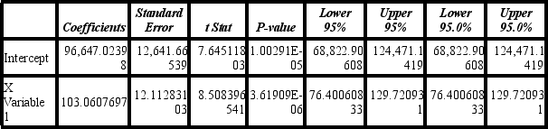
If the controller uses regression analysis to estimate costs, the cost equation for administrative costs is:
A) Administrative Costs = $19,943.58 + ($13.00 × Credit hours).
B) Administrative Costs = $69,474.40 + ($114.30 × Credit hours).
C) Administrative Costs = $96,647.02 + ($103.06 × Credit hours).
D) Administrative Costs = $12,521.26 + ($11.99 × Credit hours).
The controller's office has analyzed the data and has given you the results from the regression analysis:
-
If the controller uses regression analysis to estimate costs, the cost equation for administrative costs is:
A) Administrative Costs = $19,943.58 + ($13.00 × Credit hours).
B) Administrative Costs = $69,474.40 + ($114.30 × Credit hours).
C) Administrative Costs = $96,647.02 + ($103.06 × Credit hours).
D) Administrative Costs = $12,521.26 + ($11.99 × Credit hours).
Question
The College of Business at Northeast College is accumulating data as a first step in the preparation of next year's budget development. One cost that is being looked at closely is administrative costs as a function of student credit hours. Data on administrative costs and credit hours for the past thirteen months are shown below:
The controller's office has analyzed the data and has given you the results from the regression analysis:

-
If the controller uses regression analysis to estimate costs, the estimate of the variable portion of administrative costs is:
A) Variable Costs = $8.63 × Credit hours.
B) Variable Costs = $0.87 × Credit hours.
C) Variable Costs = $103.06 × Credit hours.
D) Variable Costs = $11.99 × Credit hours.
The controller's office has analyzed the data and has given you the results from the regression analysis:
-
If the controller uses regression analysis to estimate costs, the estimate of the variable portion of administrative costs is:
A) Variable Costs = $8.63 × Credit hours.
B) Variable Costs = $0.87 × Credit hours.
C) Variable Costs = $103.06 × Credit hours.
D) Variable Costs = $11.99 × Credit hours.
Question
Question
Question
Question
The College of Business at Northeast College is accumulating data as a first step in the preparation of next year's budget development. One cost that is being looked at closely is administrative costs as a function of student credit hours. Data on administrative costs and credit hours for the past thirteen months are shown below:
The controller's office has analyzed the data and has given you the results from the regression analysis:

-
Based on the results of the high-low analysis, the estimate of administrative costs in a month with 1,000 credit hours would be: (rounded to the nearest whole dollar)
A) $181,692.
B) $199,969.
C) $201,210.
D) $198,808.
The controller's office has analyzed the data and has given you the results from the regression analysis:
-
Based on the results of the high-low analysis, the estimate of administrative costs in a month with 1,000 credit hours would be: (rounded to the nearest whole dollar)
A) $181,692.
B) $199,969.
C) $201,210.
D) $198,808.
Question
The College of Business at Northeast College is accumulating data as a first step in the preparation of next year's budget development. One cost that is being looked at closely is administrative costs as a function of student credit hours. Data on administrative costs and credit hours for the past thirteen months are shown below:
The controller's office has analyzed the data and has given you the results from the regression analysis:

-
Based on the results of the regression analysis, the estimate of administrative costs in a month with 1,000 credit hours would be: (rounded to the nearest whole dollar)
A) $198,808.
B) $201,000.
C) $199,707.
D) $96,409.
The controller's office has analyzed the data and has given you the results from the regression analysis:
-
Based on the results of the regression analysis, the estimate of administrative costs in a month with 1,000 credit hours would be: (rounded to the nearest whole dollar)
A) $198,808.
B) $201,000.
C) $199,707.
D) $96,409.
Question
Question
The College of Business at Northeast College is accumulating data as a first step in the preparation of next year's budget development. One cost that is being looked at closely is administrative costs as a function of student credit hours. Data on administrative costs and credit hours for the past thirteen months are shown below:
The controller's office has analyzed the data and has given you the results from the regression analysis:

-
The percent of the total variance that can be explained by the regression is:
A) 93.3%.
B) 86.8%.
C) 85.9%.
D) 96.6%.
The controller's office has analyzed the data and has given you the results from the regression analysis:
-
The percent of the total variance that can be explained by the regression is:
A) 93.3%.
B) 86.8%.
C) 85.9%.
D) 96.6%.
Question
Question
Question
Question
The College of Business at Northeast College is accumulating data as a first step in the preparation of next year's budget development. One cost that is being looked at closely is administrative costs as a function of student credit hours. Data on administrative costs and credit hours for the past thirteen months are shown below:
The controller's office has analyzed the data and has given you the results from the regression analysis:

-
If the controller uses regression analysis to estimate costs, the estimate of the fixed portion of administrative costs is:
A) Fixed Cost = $103.56.
B) Fixed Cost = $12,521.26.
C) Fixed Cost = $19,943.58.
D) Fixed Cost = $96,647.02.
The controller's office has analyzed the data and has given you the results from the regression analysis:
-
If the controller uses regression analysis to estimate costs, the estimate of the fixed portion of administrative costs is:
A) Fixed Cost = $103.56.
B) Fixed Cost = $12,521.26.
C) Fixed Cost = $19,943.58.
D) Fixed Cost = $96,647.02.
Question
Question
The College of Business at Northeast College is accumulating data as a first step in the preparation of next year's budget development. One cost that is being looked at closely is administrative costs as a function of student credit hours. Data on administrative costs and credit hours for the past thirteen months are shown below:
The controller's office has analyzed the data and has given you the results from the regression analysis:

-
The correlation coefficient (rounded to the 3rd decimal) for the regression equation for administrative costs is:
A) 0.932.
B) 0.868.
C) 0.856.
D) 0.966.
The controller's office has analyzed the data and has given you the results from the regression analysis:
-
The correlation coefficient (rounded to the 3rd decimal) for the regression equation for administrative costs is:
A) 0.932.
B) 0.868.
C) 0.856.
D) 0.966.
Question
Question

Unlock Deck
Sign up to unlock the cards in this deck!
Unlock Deck
Unlock Deck
1/131
Play
Full screen (f)
Deck 5: Cost Estimation
1
A basic assumption of most cost estimation methods is cost behavior patterns are linear within the relevant range.
True
2
The linear cost estimate tends to understate the slope of the cost line in ranges close to capacity.
True
3
The relevant range represents those activity levels for which valid cost relationships have been observed.
True
4
Because outliers are extreme data points, they can be included in the regression analysis and not significantly affect the results.
Unlock Deck
Unlock for access to all 131 flashcards in this deck.
Unlock Deck
k this deck
5
In general, the account analysis method focuses on the underlying relationship between cost and activities from the previous period.
Unlock Deck
Unlock for access to all 131 flashcards in this deck.
Unlock Deck
k this deck
6
In general, cost behavior results are likely to differ between the engineering method and the account analysis method.
Unlock Deck
Unlock for access to all 131 flashcards in this deck.
Unlock Deck
k this deck
7
The engineering method of determining cost behavior is particularly useful for new activities or products.
Unlock Deck
Unlock for access to all 131 flashcards in this deck.
Unlock Deck
k this deck
8
Cost behavior is the most important characteristic for managerial decision making.
Unlock Deck
Unlock for access to all 131 flashcards in this deck.
Unlock Deck
k this deck
9
A scattergraph is useful for identifying outliers/irrelevant data points.
Unlock Deck
Unlock for access to all 131 flashcards in this deck.
Unlock Deck
k this deck
10
One way to control the effects of a nonlinear relation between total costs and volume is to reduce the relevant range.
Unlock Deck
Unlock for access to all 131 flashcards in this deck.
Unlock Deck
k this deck
11
In general, accounting records accumulate cost information according to its behavior (i.e., variable and fixed).
Unlock Deck
Unlock for access to all 131 flashcards in this deck.
Unlock Deck
k this deck
12
One disadvantage of the high-low method is the highest and lowest points may not be representative of normal operating activities.
Unlock Deck
Unlock for access to all 131 flashcards in this deck.
Unlock Deck
k this deck
13
One advantage of the engineering method is that it does not require data from prior periods to estimate cost behavior.
Unlock Deck
Unlock for access to all 131 flashcards in this deck.
Unlock Deck
k this deck
14
Different cost estimations methods may produce different cost equations, even when using the same set of data.
Unlock Deck
Unlock for access to all 131 flashcards in this deck.
Unlock Deck
k this deck
15
Cost estimates using regression analysis are always more accurate and dependable than cost estimates using the scattergraph methods.
Unlock Deck
Unlock for access to all 131 flashcards in this deck.
Unlock Deck
k this deck
16
The quality of the cost equation depends on collecting appropriate data.
Unlock Deck
Unlock for access to all 131 flashcards in this deck.
Unlock Deck
k this deck
17
The account analysis method is more subjective than other cost estimation methods because it relies heavily on the personal judgment and experience of accountants.
Unlock Deck
Unlock for access to all 131 flashcards in this deck.
Unlock Deck
k this deck
18
In general, the use of multiple independent variables increases the proportion of the variation in the dependent variable explained by the cost equation.
Unlock Deck
Unlock for access to all 131 flashcards in this deck.
Unlock Deck
k this deck
19
One advantage of the account analysis method for estimating cost behavior is that it includes actual work conditions.
Unlock Deck
Unlock for access to all 131 flashcards in this deck.
Unlock Deck
k this deck
20
One advantage that regression techniques have over other cost estimation methods is it generates information that can be used to determine how well the estimated cost equation will predict future costs.
Unlock Deck
Unlock for access to all 131 flashcards in this deck.
Unlock Deck
k this deck
21
Which of the following is not true of regression techniques for estimating costs?
A) They permit the inclusion of more than one predictor.
B) They typically use the highest and lowest activity points to estimate the relation between cost and activity.
C) They help develop estimates that have a broader base than those based on a few select points.
D) They are designed to generate a line that best fits a set of data points.
Unlock Deck
Unlock for access to all 131 flashcards in this deck.
Unlock Deck
k this deck
22
Which of the following statements is(are) true regarding cost behaviors?
(A) In general, accounting records accumulate cost information according to its behavior.
(B) Cost behaviors are the most important consideration in managerial decision making.
A) Only A is true.
B) Only B is true.
C) Both of these are true.
D) Neither of these is true.
(A) In general, accounting records accumulate cost information according to its behavior.
(B) Cost behaviors are the most important consideration in managerial decision making.
A) Only A is true.
B) Only B is true.
C) Both of these are true.
D) Neither of these is true.
Unlock Deck
Unlock for access to all 131 flashcards in this deck.
Unlock Deck
k this deck
23
Which of the following costs would most likely be classified as variable, assuming the account analysis method is used to determine cost behaviors?
A) Indirect materials.
B) Supervisory salaries.
C) Equipment maintenance.
D) Building occupancy costs.
A) Indirect materials.
B) Supervisory salaries.
C) Equipment maintenance.
D) Building occupancy costs.
Unlock Deck
Unlock for access to all 131 flashcards in this deck.
Unlock Deck
k this deck
24
The term "relevant range," as used in cost accounting, means the range over which:
A) relevant costs are incurred.
B) costs may fluctuate.
C) cost relationships are valid.
D) cost data is available.
A) relevant costs are incurred.
B) costs may fluctuate.
C) cost relationships are valid.
D) cost data is available.
Unlock Deck
Unlock for access to all 131 flashcards in this deck.
Unlock Deck
k this deck
25
Which of the following is the difference between variable costs and fixed costs? (CMA adapted)
A) Variable costs per unit fluctuate and fixed costs per unit remain constant.
B) Variable costs per unit are fixed over the relevant range and fixed costs per unit are variable.
C) Total variable costs are variable over the relevant range and fixed in the long term, while fixed costs never change.
D) Variable costs per unit change in varying increments, while fixed costs per unit change in equal units.
Unlock Deck
Unlock for access to all 131 flashcards in this deck.
Unlock Deck
k this deck
26
The correlation coefficient is:
A) the range of values over which the probability may be estimated based upon the regression equation results.
B) the proportion of the total variance in the dependent variable explained by the independent variable.
C) the measure of variability of the actual observations from the predicting (forecasting) equation line.
D) the relative degree that changes in one variable can be used to estimate changes in another variable.
Unlock Deck
Unlock for access to all 131 flashcards in this deck.
Unlock Deck
k this deck
27
Which of the following cost estimation methods is based on two cost observations?
A) Engineering approach.
B) High-low method.
C) Account analysis.
D) Linear regression.
A) Engineering approach.
B) High-low method.
C) Account analysis.
D) Linear regression.
Unlock Deck
Unlock for access to all 131 flashcards in this deck.
Unlock Deck
k this deck
28
Ballard Company incurred a total cost of $8,600 to produce 400 units of pulp. Each unit of pulp required five (5) direct labor hours to complete. What is the total fixed cost if the variable cost was $1.50 per direct labor hour?
A) $1,700.
B) $3,000.
C) $5,600.
D) $8,000.
A) $1,700.
B) $3,000.
C) $5,600.
D) $8,000.
Unlock Deck
Unlock for access to all 131 flashcards in this deck.
Unlock Deck
k this deck
29
Brewsky's is a chain of micro-breweries. Managers are interested in the costs of the stores and believe that the costs can be explained in large part by the number of customers patronizing the stores. Monthly data regarding customer visits and costs for the preceding year for one of the stores have been entered into the regression analysis and the analysis is as follows:
-
In a regression equation expressed as y = a + bx, how is the letter b best described? (CMA adapted)
A) An estimate of the probability of return customers.
B) The fixed costs per customer visit.
C) The estimate of the cost for an additional customer visit.
D) The proximity of the data points to the regression line.
Unlock Deck
Unlock for access to all 131 flashcards in this deck.
Unlock Deck
k this deck
30
Given the following information, compute the total number of units for the period:
A) 360.
B) 432.
C) 640.
D) 840.
A) 360.
B) 432.
C) 640.
D) 840.
Unlock Deck
Unlock for access to all 131 flashcards in this deck.
Unlock Deck
k this deck
31
Which cost estimation method does not use the company's cost information as its primary source of information about the relationship between total costs and activity levels?
A) Scattergraph.
B) High-low.
C) Account analysis.
D) Engineering estimates.
A) Scattergraph.
B) High-low.
C) Account analysis.
D) Engineering estimates.
Unlock Deck
Unlock for access to all 131 flashcards in this deck.
Unlock Deck
k this deck
32
In the cost equation TC = F + VX, "V" is best described as the:
A) total costs that do not vary with changes in the activity level.
B) intercept of the cost equation.
C) slope of the cost equation.
D) activity level used to estimate the dependent variable.
A) total costs that do not vary with changes in the activity level.
B) intercept of the cost equation.
C) slope of the cost equation.
D) activity level used to estimate the dependent variable.
Unlock Deck
Unlock for access to all 131 flashcards in this deck.
Unlock Deck
k this deck
33
A manager is trying to estimate the manufacturing costs of a new product. The company makes several other products that utilize some of the same manufacturing procedures as the new product. Which cost estimation method would be the best method to determine the total cost of manufacturing the new product?
A) Engineering estimates.
B) Regression analysis.
C) Account analysis.
D) Scattergraph.
A) Engineering estimates.
B) Regression analysis.
C) Account analysis.
D) Scattergraph.
Unlock Deck
Unlock for access to all 131 flashcards in this deck.
Unlock Deck
k this deck
34
Identifying the relation between the activity and the costs is a key step in which of the following cost estimation methods?
A) Scattergraph.
B) High-low method.
C) Account analysis.
D) Linear regression.
A) Scattergraph.
B) High-low method.
C) Account analysis.
D) Linear regression.
Unlock Deck
Unlock for access to all 131 flashcards in this deck.
Unlock Deck
k this deck
35
Obtaining regression estimates for cost estimation requires establishing the existence of a logical relation between activities and the cost to be estimated. Which of the following is not used to refer to the cost to be estimated?
A) left-hand side (LHS).
B) dependent variable.
C) Y term.
D) independent variable.
A) left-hand side (LHS).
B) dependent variable.
C) Y term.
D) independent variable.
Unlock Deck
Unlock for access to all 131 flashcards in this deck.
Unlock Deck
k this deck
36
In the cost equation TC = F + VX, "X" is best described as the:
A) costs that do not vary with changes in the activity level.
B) costs that do vary with changes in the activity level.
C) total cost estimate at a particular activity level.
D) activity level used to estimate the total cost.
A) costs that do not vary with changes in the activity level.
B) costs that do vary with changes in the activity level.
C) total cost estimate at a particular activity level.
D) activity level used to estimate the total cost.
Unlock Deck
Unlock for access to all 131 flashcards in this deck.
Unlock Deck
k this deck
37
Obtaining regression estimates for cost estimation requires establishing the existence of a logical relation between activities and the cost to be estimated. Which of the following is not used to refer to these activities?
A) independent variables.
B) predictors.
C) dependent variables.
D) X terms.
A) independent variables.
B) predictors.
C) dependent variables.
D) X terms.
Unlock Deck
Unlock for access to all 131 flashcards in this deck.
Unlock Deck
k this deck
38
Engineering cost estimates are usually based on operating conditions that are considered:
A) optimal.
B) practical.
C) attainable.
D) historical.
A) optimal.
B) practical.
C) attainable.
D) historical.
Unlock Deck
Unlock for access to all 131 flashcards in this deck.
Unlock Deck
k this deck
39
A disadvantage of the high-low method of cost analysis is that it:
A) typically results in a totally inaccurate cost formula.
B) is too time consuming to apply.
C) uses only two data points, which may not be representative of normal conditions.
D) relies totally on the judgment of the person performing the cost analysis.
A) typically results in a totally inaccurate cost formula.
B) is too time consuming to apply.
C) uses only two data points, which may not be representative of normal conditions.
D) relies totally on the judgment of the person performing the cost analysis.
Unlock Deck
Unlock for access to all 131 flashcards in this deck.
Unlock Deck
k this deck
40
A cost driver is defined as: (CMA adapted)
A) the largest cost in a manufacturing process.
B) a fixed cost that cannot be avoided.
C) the significant factor in developing a new product.
D) a causal factor that increases the total cost of a cost objective.
A) the largest cost in a manufacturing process.
B) a fixed cost that cannot be avoided.
C) the significant factor in developing a new product.
D) a causal factor that increases the total cost of a cost objective.
Unlock Deck
Unlock for access to all 131 flashcards in this deck.
Unlock Deck
k this deck
41
The College of Business at Northeast College is accumulating data as a first step in the preparation of next year's budget development. One cost that is being looked at closely is administrative costs as a function of student credit hours. Data on administrative costs and credit hours for the past thirteen months are shown below:
The controller's office has analyzed the data and has given you the results from the regression analysis:
-
If the controller uses the high-low method to estimate costs, the fixed cost portion of the cost equation for administrative costs is:
A) $198,808.00.
B) $69,731.68.
C) $96,409.42.
D) $19,943.58.
Unlock Deck
Unlock for access to all 131 flashcards in this deck.
Unlock Deck
k this deck
42
Brewsky's is a chain of micro-breweries. Managers are interested in the costs of the stores and believe that the costs can be explained in large part by the number of customers patronizing the stores. Monthly data regarding customer visits and costs for the preceding year for one of the stores have been entered into the regression analysis and the analysis is as follows:
-
What is the percent of the total variance that can be explained by the regression equation? (CMA adapted)
A) 86.8%
B) 31.6%
C) 97.7%
D) 71.9%
-
What is the percent of the total variance that can be explained by the regression equation? (CMA adapted)
A) 86.8%
B) 31.6%
C) 97.7%
D) 71.9%
Unlock Deck
Unlock for access to all 131 flashcards in this deck.
Unlock Deck
k this deck
43
The McGraw Company is accumulating data to be used in preparing its annual profit plan for the coming year. The cost behavior pattern of the maintenance costs must be determined. The accounting staff has suggested that linear regression be employed to derive an equation in the form of y = a + bx for maintenance costs. Data regarding the maintenance hours and costs for last year and the results of the regression analysis are as follows: (CMA adapted)
-Based upon the data derived from the regression analysis, 420 maintenance hours in a month would mean the maintenance costs would be budgeted at: (rounded to the nearest whole dollar)
A) $3,797.
B) $3,780.
C) $3,746.
D) $3,600.
-Based upon the data derived from the regression analysis, 420 maintenance hours in a month would mean the maintenance costs would be budgeted at: (rounded to the nearest whole dollar)
A) $3,797.
B) $3,780.
C) $3,746.
D) $3,600.
Unlock Deck
Unlock for access to all 131 flashcards in this deck.
Unlock Deck
k this deck
44
Fromme's Frocks has the following machine hours and production costs for the last six months of last year:
If Fromme expects to incur 14,000 machine hours in January, what will be the estimated total production cost using the high-low method?
A) $8,750.00.
B) $11,142.50.
C) $22,400.00.
D) $10,889.10.
If Fromme expects to incur 14,000 machine hours in January, what will be the estimated total production cost using the high-low method?
A) $8,750.00.
B) $11,142.50.
C) $22,400.00.
D) $10,889.10.
Unlock Deck
Unlock for access to all 131 flashcards in this deck.
Unlock Deck
k this deck
45
The controller of Fortnight Co. has requested a quick estimate of the manufacturing supplies needed for the Cleveland Plant for the month of July, when production is expected to be 470,000 units to meet the ending inventory requirements and sales of 475,000 units. Fortnight Co.'s budget analyst has the following actual data for the last three months.
Using the high-low method to develop a cost estimating equation, the total estimated cost of needed manufacturing supplies for July would be: (CMA adapted)
A) $681,500.
B) $688,750.
C) $749,180.
D) $752,060.
Using the high-low method to develop a cost estimating equation, the total estimated cost of needed manufacturing supplies for July would be: (CMA adapted)
A) $681,500.
B) $688,750.
C) $749,180.
D) $752,060.
Unlock Deck
Unlock for access to all 131 flashcards in this deck.
Unlock Deck
k this deck
46
The McGraw Company is accumulating data to be used in preparing its annual profit plan for the coming year. The cost behavior pattern of the maintenance costs must be determined. The accounting staff has suggested that linear regression be employed to derive an equation in the form of y = a + bx for maintenance costs. Data regarding the maintenance hours and costs for last year and the results of the regression analysis are as follows: (CMA adapted)
- What is the fixed cost per month using the high-low method to estimate the cost equation?
A) $570.
B) $600.
C) $1,140.
D) $2,250.
- What is the fixed cost per month using the high-low method to estimate the cost equation?
A) $570.
B) $600.
C) $1,140.
D) $2,250.
Unlock Deck
Unlock for access to all 131 flashcards in this deck.
Unlock Deck
k this deck
47
The Crater Manufacturing Company recorded overhead costs of $14,182 at an activity level of 4,200 machine hours and $8,748 at 2,300 machine hours. The records also indicated that overhead of $9,730 was incurred at 2,600 machine hours. What is the variable cost per machine hour using the high-low method to estimate the cost equation?
A) $2.78.
B) $2.86.
C) $3.10.
D) $3.38.
A) $2.78.
B) $2.86.
C) $3.10.
D) $3.38.
Unlock Deck
Unlock for access to all 131 flashcards in this deck.
Unlock Deck
k this deck
48
Brewsky's is a chain of micro-breweries. Managers are interested in the costs of the stores and believe that the costs can be explained in large part by the number of customers patronizing the stores. Monthly data regarding customer visits and costs for the preceding year for one of the stores have been entered into the regression analysis and the analysis is as follows:
-
Based on the data derived from the regression analysis, what are the estimated costs for 1,600 customer visits in a month? (CMA adapted)
A) $6,125.
B) $4,629.
C) $3,328.
D) $4,824.
-
Based on the data derived from the regression analysis, what are the estimated costs for 1,600 customer visits in a month? (CMA adapted)
A) $6,125.
B) $4,629.
C) $3,328.
D) $4,824.
Unlock Deck
Unlock for access to all 131 flashcards in this deck.
Unlock Deck
k this deck
49
Brewsky's is a chain of micro-breweries. Managers are interested in the costs of the stores and believe that the costs can be explained in large part by the number of customers patronizing the stores. Monthly data regarding customer visits and costs for the preceding year for one of the stores have been entered into the regression analysis and the analysis is as follows:
-
In a regression equation expressed as y = a + bx, how is the letter y best described? (CMA adapted)
A) An estimate of the total customers for the month.
B) The observed store cost for a given month.
C) The estimate of the number of new customer visits for the month.
D) The proximity of the data points to the regression line.
Unlock Deck
Unlock for access to all 131 flashcards in this deck.
Unlock Deck
k this deck
50
The McGraw Company is accumulating data to be used in preparing its annual profit plan for the coming year. The cost behavior pattern of the maintenance costs must be determined. The accounting staff has suggested that linear regression be employed to derive an equation in the form of y = a + bx for maintenance costs. Data regarding the maintenance hours and costs for last year and the results of the regression analysis are as follows: (CMA adapted)
- What would be the cost equation if the high-low method is used?
A) Maintenance Costs = $9.00 × Hours of Activity.
B) Maintenance Costs = 3,600 + (400 × Hours of Activity).
C) Maintenance Costs = $570 + ($7.50 × Hours of Activity).
D) Maintenance Costs = $34.469 + ($0.99724 × Hours of Activity).
- What would be the cost equation if the high-low method is used?
A) Maintenance Costs = $9.00 × Hours of Activity.
B) Maintenance Costs = 3,600 + (400 × Hours of Activity).
C) Maintenance Costs = $570 + ($7.50 × Hours of Activity).
D) Maintenance Costs = $34.469 + ($0.99724 × Hours of Activity).
Unlock Deck
Unlock for access to all 131 flashcards in this deck.
Unlock Deck
k this deck
51
The College of Business at Northeast College is accumulating data as a first step in the preparation of next year's budget development. One cost that is being looked at closely is administrative costs as a function of student credit hours. Data on administrative costs and credit hours for the past thirteen months are shown below:
The controller's office has analyzed the data and has given you the results from the regression analysis:
-
If the controller uses the high-low method to estimate costs, the variable cost per credit hour is:
A) $82.33.
B) $103.56.
C) $111.96.
D) $201.22.
The controller's office has analyzed the data and has given you the results from the regression analysis:
-
If the controller uses the high-low method to estimate costs, the variable cost per credit hour is:
A) $82.33.
B) $103.56.
C) $111.96.
D) $201.22.
Unlock Deck
Unlock for access to all 131 flashcards in this deck.
Unlock Deck
k this deck
52
The McGraw Company is accumulating data to be used in preparing its annual profit plan for the coming year. The cost behavior pattern of the maintenance costs must be determined. The accounting staff has suggested that linear regression be employed to derive an equation in the form of y = a + bx for maintenance costs. Data regarding the maintenance hours and costs for last year and the results of the regression analysis are as follows: (CMA adapted)
-What is the variable cost per hour using the high-low method to estimate the cost equation?
A) $9.00.
B) $7.50.
C) $0.1333.
D) $0.1111.
-What is the variable cost per hour using the high-low method to estimate the cost equation?
A) $9.00.
B) $7.50.
C) $0.1333.
D) $0.1111.
Unlock Deck
Unlock for access to all 131 flashcards in this deck.
Unlock Deck
k this deck
53
The McGraw Company is accumulating data to be used in preparing its annual profit plan for the coming year. The cost behavior pattern of the maintenance costs must be determined. The accounting staff has suggested that linear regression be employed to derive an equation in the form of y = a + bx for maintenance costs. Data regarding the maintenance hours and costs for last year and the results of the regression analysis are as follows: (CMA adapted)
-What would be the cost equation if regression analysis is used?
A) Maintenance Costs = $7.2884 + ($684.65 × Hours of Activity).
B) Maintenance Costs = $684.65 + ($49.515 × Hours of Activity).
C) Maintenance Costs = $684.65 + ($7.2884 × Hours of Activity).
D) Maintenance Costs = $34.469 + ($0.99724 × Hours of Activity).
Unlock Deck
Unlock for access to all 131 flashcards in this deck.
Unlock Deck
k this deck
54
The Missou Manufacturing Company recorded overhead costs of $14,182 at an activity level of 4,200 machine hours and $8,748 at 2,300 machine hours. What is the total estimated cost for 2,600 machine hours using the high-low method to estimate the cost equation?
A) $9,730.
B) $9,606.
C) $9,106.
D) $8,788.
A) $9,730.
B) $9,606.
C) $9,106.
D) $8,788.
Unlock Deck
Unlock for access to all 131 flashcards in this deck.
Unlock Deck
k this deck
55
Brewsky's is a chain of micro-breweries. Managers are interested in the costs of the stores and believe that the costs can be explained in large part by the number of customers patronizing the stores. Monthly data regarding customer visits and costs for the preceding year for one of the stores have been entered into the regression analysis and the analysis is as follows:
-
In a regression equation expressed as y = a + bx, how is the letter x best described? (CMA adapted)
A) Fixed costs per each customer-visit.
B) The observed store costs for a given month.
C) The estimate of the number of new customer visits for the month.
D) The observed customer visits for a given month.
Unlock Deck
Unlock for access to all 131 flashcards in this deck.
Unlock Deck
k this deck
56
The College of Business at Northeast College is accumulating data as a first step in the preparation of next year's budget development. One cost that is being looked at closely is administrative costs as a function of student credit hours. Data on administrative costs and credit hours for the past thirteen months are shown below:
The controller's office has analyzed the data and has given you the results from the regression analysis:
-
If the controller uses the high-low method to estimate costs, the cost equation for administrative costs is
A) Administrative Costs = $96,409.42 + $103.56 × Credit-hours.
B) Administrative Costs = $69,731.68 + $111.96 × Credit-hours.
C) Administrative Costs = $201.21 × Credit-hours.
D) Administrative Costs = $198,808.
Unlock Deck
Unlock for access to all 131 flashcards in this deck.
Unlock Deck
k this deck
57
The Macon Company uses the high-low method to determine its cost equation. The following information was gathered for the past year:
-
If Macon expects to use 10,000 machine hours next month, what are the estimated direct labor costs?
A) $160,000.
B) $180,000.
C) $175,000.
D) $150,000.
-
If Macon expects to use 10,000 machine hours next month, what are the estimated direct labor costs?
A) $160,000.
B) $180,000.
C) $175,000.
D) $150,000.
Unlock Deck
Unlock for access to all 131 flashcards in this deck.
Unlock Deck
k this deck
58
The Macon Company uses the high-low method to determine its cost equation. The following information was gathered for the past year:
-
What are the direct labor costs per machine hour?
A) $20.00.
B) $16.00.
C) $14.29.
D) $10.00.
-
What are the direct labor costs per machine hour?
A) $20.00.
B) $16.00.
C) $14.29.
D) $10.00.
Unlock Deck
Unlock for access to all 131 flashcards in this deck.
Unlock Deck
k this deck
59
The McGraw Company is accumulating data to be used in preparing its annual profit plan for the coming year. The cost behavior pattern of the maintenance costs must be determined. The accounting staff has suggested that linear regression be employed to derive an equation in the form of y = a + bx for maintenance costs. Data regarding the maintenance hours and costs for last year and the results of the regression analysis are as follows: (CMA adapted)
-Using the high-low method to estimate cost behavior, 420 maintenance hours in a month would mean the maintenance costs would be budgeted at:
A) $3,150.
B) $3,600.
C) $3,720.
D) $3,780.
-Using the high-low method to estimate cost behavior, 420 maintenance hours in a month would mean the maintenance costs would be budgeted at:
A) $3,150.
B) $3,600.
C) $3,720.
D) $3,780.
Unlock Deck
Unlock for access to all 131 flashcards in this deck.
Unlock Deck
k this deck
60
The cost accountants at the Barkley Company regressed total overhead costs and direct labor hours for the past 30-months and reported the following results:
What is the estimated overhead cost if 225 direct labor hours are expected to be used in the upcoming period? (rounded to the nearest whole dollar)
A) $10,534.
B) $9,882.
C) $9,230.
D) $8,617.
What is the estimated overhead cost if 225 direct labor hours are expected to be used in the upcoming period? (rounded to the nearest whole dollar)
A) $10,534.
B) $9,882.
C) $9,230.
D) $8,617.
Unlock Deck
Unlock for access to all 131 flashcards in this deck.
Unlock Deck
k this deck
61
Thane Company is interested in establishing the relationship between electricity costs and machine hours. Data have been collected and a regression analysis prepared using Excel. The monthly data and the regression output follow:
-
If the controller uses the high-low method to estimate costs, the variable cost per machine hour is:
A) $6.25.
B) $6.90.
C) $5.77.
D) $11.70.
-
If the controller uses the high-low method to estimate costs, the variable cost per machine hour is:
A) $6.25.
B) $6.90.
C) $5.77.
D) $11.70.
Unlock Deck
Unlock for access to all 131 flashcards in this deck.
Unlock Deck
k this deck
62
The College of Business at Northeast College is accumulating data as a first step in the preparation of next year's budget development. One cost that is being looked at closely is administrative costs as a function of student credit hours. Data on administrative costs and credit hours for the past thirteen months are shown below:
The controller's office has analyzed the data and has given you the results from the regression analysis:
-
Based on the results of the regression analysis, the estimate of the variable portion of administrative costs in a month with 200 credit hours would be:
A) $198,808.
B) $20,612.
C) $117,121.
D) $40,242.
Unlock Deck
Unlock for access to all 131 flashcards in this deck.
Unlock Deck
k this deck
63
Thane Company is interested in establishing the relationship between electricity costs and machine hours. Data have been collected and a regression analysis prepared using Excel. The monthly data and the regression output follow:
-
Based on the results of the high-low analysis, the estimate of electricity costs in a month with 2,200 machine hours would be:
A) $15,375.
B) $22,825.
C) $15,180.
D) $16,427.
-
Based on the results of the high-low analysis, the estimate of electricity costs in a month with 2,200 machine hours would be:
A) $15,375.
B) $22,825.
C) $15,180.
D) $16,427.
Unlock Deck
Unlock for access to all 131 flashcards in this deck.
Unlock Deck
k this deck
64
The College of Business at Northeast College is accumulating data as a first step in the preparation of next year's budget development. One cost that is being looked at closely is administrative costs as a function of student credit hours. Data on administrative costs and credit hours for the past thirteen months are shown below:
The controller's office has analyzed the data and has given you the results from the regression analysis:
-
If the controller uses regression analysis to estimate costs, the cost equation for administrative costs is:
A) Administrative Costs = $19,943.58 + ($13.00 × Credit hours).
B) Administrative Costs = $69,474.40 + ($114.30 × Credit hours).
C) Administrative Costs = $96,647.02 + ($103.06 × Credit hours).
D) Administrative Costs = $12,521.26 + ($11.99 × Credit hours).
Unlock Deck
Unlock for access to all 131 flashcards in this deck.
Unlock Deck
k this deck
65
The College of Business at Northeast College is accumulating data as a first step in the preparation of next year's budget development. One cost that is being looked at closely is administrative costs as a function of student credit hours. Data on administrative costs and credit hours for the past thirteen months are shown below:
The controller's office has analyzed the data and has given you the results from the regression analysis:
-
If the controller uses regression analysis to estimate costs, the estimate of the variable portion of administrative costs is:
A) Variable Costs = $8.63 × Credit hours.
B) Variable Costs = $0.87 × Credit hours.
C) Variable Costs = $103.06 × Credit hours.
D) Variable Costs = $11.99 × Credit hours.
Unlock Deck
Unlock for access to all 131 flashcards in this deck.
Unlock Deck
k this deck
66
In determining cost behavior in business, the cost function is often expressed as Y = a + bX. Which one of the following cost estimation methods should not be used in estimating fixed and variable costs for the equation? (CMA adapted)
A) Scattergraph method.
B) Simple regression.
C) High and low point method.
D) Management analysis of data.
A) Scattergraph method.
B) Simple regression.
C) High and low point method.
D) Management analysis of data.
Unlock Deck
Unlock for access to all 131 flashcards in this deck.
Unlock Deck
k this deck
67
Thane Company is interested in establishing the relationship between electricity costs and machine hours. Data have been collected and a regression analysis prepared using Excel. The monthly data and the regression output follow:
-
The correlation coefficient for the regression equation for electricity costs is:
A) 0.965.
B) 0.932.
C) 0.925.
D) 0.982.
-
The correlation coefficient for the regression equation for electricity costs is:
A) 0.965.
B) 0.932.
C) 0.925.
D) 0.982.
Unlock Deck
Unlock for access to all 131 flashcards in this deck.
Unlock Deck
k this deck
68
Thane Company is interested in establishing the relationship between electricity costs and machine hours. Data have been collected and a regression analysis prepared using Excel. The monthly data and the regression output follow:
-
The percent of the total variance that can be explained by the regression is:
A) 96.5%.
B) 93.2%.
C) 92.5%.
D) 98.2%.
-
The percent of the total variance that can be explained by the regression is:
A) 96.5%.
B) 93.2%.
C) 92.5%.
D) 98.2%.
Unlock Deck
Unlock for access to all 131 flashcards in this deck.
Unlock Deck
k this deck
69
The College of Business at Northeast College is accumulating data as a first step in the preparation of next year's budget development. One cost that is being looked at closely is administrative costs as a function of student credit hours. Data on administrative costs and credit hours for the past thirteen months are shown below:
The controller's office has analyzed the data and has given you the results from the regression analysis:
-
Based on the results of the high-low analysis, the estimate of administrative costs in a month with 1,000 credit hours would be: (rounded to the nearest whole dollar)
A) $181,692.
B) $199,969.
C) $201,210.
D) $198,808.
Unlock Deck
Unlock for access to all 131 flashcards in this deck.
Unlock Deck
k this deck
70
The College of Business at Northeast College is accumulating data as a first step in the preparation of next year's budget development. One cost that is being looked at closely is administrative costs as a function of student credit hours. Data on administrative costs and credit hours for the past thirteen months are shown below:
The controller's office has analyzed the data and has given you the results from the regression analysis:
-
Based on the results of the regression analysis, the estimate of administrative costs in a month with 1,000 credit hours would be: (rounded to the nearest whole dollar)
A) $198,808.
B) $201,000.
C) $199,707.
D) $96,409.
Unlock Deck
Unlock for access to all 131 flashcards in this deck.
Unlock Deck
k this deck
71
Which of the following may be used to estimate how inventory warehouse costs are affected by both the number of shipments and the weight of the material handled? (CPA adapted)
A) Economic order quantity analysis.
B) Probability analysis.
C) Correlation analysis.
D) Multiple regression analysis.
A) Economic order quantity analysis.
B) Probability analysis.
C) Correlation analysis.
D) Multiple regression analysis.
Unlock Deck
Unlock for access to all 131 flashcards in this deck.
Unlock Deck
k this deck
72
The College of Business at Northeast College is accumulating data as a first step in the preparation of next year's budget development. One cost that is being looked at closely is administrative costs as a function of student credit hours. Data on administrative costs and credit hours for the past thirteen months are shown below:
The controller's office has analyzed the data and has given you the results from the regression analysis:
-
The percent of the total variance that can be explained by the regression is:
A) 93.3%.
B) 86.8%.
C) 85.9%.
D) 96.6%.
The controller's office has analyzed the data and has given you the results from the regression analysis:
-
The percent of the total variance that can be explained by the regression is:
A) 93.3%.
B) 86.8%.
C) 85.9%.
D) 96.6%.
Unlock Deck
Unlock for access to all 131 flashcards in this deck.
Unlock Deck
k this deck
73
Thane Company is interested in establishing the relationship between electricity costs and machine hours. Data have been collected and a regression analysis prepared using Excel. The monthly data and the regression output follow:
-
If the controller uses regression analysis to estimate costs, the estimate of the variable portion of electricity costs is:
A) Electricity Costs = $11.70 × Machine hours.
B) Electricity Costs = $0.93 × Machine hours.
C) Electricity Costs = $5.77 × Machine hours.
D) Electricity Costs = $0.49 × Machine hours.
Unlock Deck
Unlock for access to all 131 flashcards in this deck.
Unlock Deck
k this deck
74
Thane Company is interested in establishing the relationship between electricity costs and machine hours. Data have been collected and a regression analysis prepared using Excel. The monthly data and the regression output follow:
-
Based on the results of the regression analysis, the estimate of electricity costs in a month with 2,200 machine hours would be: (rounded to the nearest whole dollar)
A) $3,727.
B) $16,421.
C) $15,180.
D) $22,825.
-
Based on the results of the regression analysis, the estimate of electricity costs in a month with 2,200 machine hours would be: (rounded to the nearest whole dollar)
A) $3,727.
B) $16,421.
C) $15,180.
D) $22,825.
Unlock Deck
Unlock for access to all 131 flashcards in this deck.
Unlock Deck
k this deck
75
Thane Company is interested in establishing the relationship between electricity costs and machine hours. Data have been collected and a regression analysis prepared using Excel. The monthly data and the regression output follow:
-
If the controller uses regression analysis to estimate costs, the estimate of the fixed portion of electricity costs is:
A) Fixed Cost = $5.77.
B) Fixed Cost = $1,682.82.
C) Fixed Cost = $1,425.18.
D) Fixed Cost = $3,726.88
-
If the controller uses regression analysis to estimate costs, the estimate of the fixed portion of electricity costs is:
A) Fixed Cost = $5.77.
B) Fixed Cost = $1,682.82.
C) Fixed Cost = $1,425.18.
D) Fixed Cost = $3,726.88
Unlock Deck
Unlock for access to all 131 flashcards in this deck.
Unlock Deck
k this deck
76
The College of Business at Northeast College is accumulating data as a first step in the preparation of next year's budget development. One cost that is being looked at closely is administrative costs as a function of student credit hours. Data on administrative costs and credit hours for the past thirteen months are shown below:
The controller's office has analyzed the data and has given you the results from the regression analysis:
-
If the controller uses regression analysis to estimate costs, the estimate of the fixed portion of administrative costs is:
A) Fixed Cost = $103.56.
B) Fixed Cost = $12,521.26.
C) Fixed Cost = $19,943.58.
D) Fixed Cost = $96,647.02.
Unlock Deck
Unlock for access to all 131 flashcards in this deck.
Unlock Deck
k this deck
77
Thane Company is interested in establishing the relationship between electricity costs and machine hours. Data have been collected and a regression analysis prepared using Excel. The monthly data and the regression output follow:
-
If the controller uses regression analysis to estimate costs, the cost equation for electricity costs is:
A) Electricity Costs = $1,425.18 + ($12.00 × Machine hours).
B) Electricity Costs = $3,726.88 + ($1,682.82 × Machine hours).
C) Electricity Costs = $1,682.82 + ($0.49 × Machine hours).
D) Electricity Costs = $3,726.88 + ($5.77 × Machine hours).
Unlock Deck
Unlock for access to all 131 flashcards in this deck.
Unlock Deck
k this deck
78
The College of Business at Northeast College is accumulating data as a first step in the preparation of next year's budget development. One cost that is being looked at closely is administrative costs as a function of student credit hours. Data on administrative costs and credit hours for the past thirteen months are shown below:
The controller's office has analyzed the data and has given you the results from the regression analysis:
-
The correlation coefficient (rounded to the 3rd decimal) for the regression equation for administrative costs is:
A) 0.932.
B) 0.868.
C) 0.856.
D) 0.966.
The controller's office has analyzed the data and has given you the results from the regression analysis:
-
The correlation coefficient (rounded to the 3rd decimal) for the regression equation for administrative costs is:
A) 0.932.
B) 0.868.
C) 0.856.
D) 0.966.
Unlock Deck
Unlock for access to all 131 flashcards in this deck.
Unlock Deck
k this deck
79
Thane Company is interested in establishing the relationship between electricity costs and machine hours. Data have been collected and a regression analysis prepared using Excel. The monthly data and the regression output follow:
-
If the controller uses the high-low method to estimate costs, the fixed cost portion of the cost equation for electricity costs is:
A) $3,726.88.
B) $1,425.18.
C) $1,625.00.
D) $22,825.00.
-
If the controller uses the high-low method to estimate costs, the fixed cost portion of the cost equation for electricity costs is:
A) $3,726.88.
B) $1,425.18.
C) $1,625.00.
D) $22,825.00.
Unlock Deck
Unlock for access to all 131 flashcards in this deck.
Unlock Deck
k this deck
80
Thane Company is interested in establishing the relationship between electricity costs and machine hours. Data have been collected and a regression analysis prepared using Excel. The monthly data and the regression output follow:
-
If the controller uses the high-low method to estimate costs, the cost equation for electricity costs is:
A) Electricity Costs = $3,726.88 + ($5.77 × Machine-hours).
B) Electricity Costs = $1,625.00 + ($6.25 × Machine-hours).
C) Electricity Costs = $6.90 × Machine-hours.
D) Electricity Costs = $22,825.
Unlock Deck
Unlock for access to all 131 flashcards in this deck.
Unlock Deck
k this deck
Unlock Deck
Unlock for access to all 131 flashcards in this deck.


