Intermediate Microeconomics and Its Application 12th Edition by Walter Nicholson,Christopher Snyder

Exercise 17

Marshall defined an equilibrium price as one at which the quantity demanded equals the quantity supplied.
a. Using the data provided in problem, show that P = 3 is the equilibrium price in the orange juice market.
b. Using these data, explain why P = 2 and P = 4 are not equilibrium prices.
c. Graph your results and show that the supply demand equilibrium resembles that shown in Figure.
d. Suppose the demand for orange juice were to increase so that people want to buy 300 million more gallons at every price. How would that change the data in problem? How would it shift the demand curve you drew in part c?
e. What is the new equilibrium price in the orange juice market, given this increase in demand? Show this new equilibrium in your supply demand graph.
f. Suppose now that a freeze in Florida reduces orange juice supply by 300 million gallons at every price listed in problem How would this shift in supply affect the data in problem? How would it affect the algebraic supply curve calculated in that problem?
g. Given this new supply relationship together with the demand relationship shown in problem, what is the equilibrium price in this market?
h. Explain why P = 3 is no longer an equilibrium in the orange juice market. How would the participants in this market know P = 3 is no longer an equilibrium?
i. Graph your results for this supply shift.
Problerm The following data represent 5 points on the supply curve for orange juice: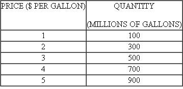 and these data represent 5 points on the demand curve for orange juice: 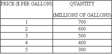a. Graph the points of these supply and demand curves for orange juice. Be sure to put price on the vertical axis and quantity on the horizontal axis.
b. Do these points seem to lie along two straight lines? If so, figure out the precise algebraic equation of these lines. (Hint: If the points do lie on straight lines, you need only consider two points on each of them to calculate the lines.)c. Use your solutions from part b to calculate the "excess demand" for orange juice if the market price is zero.
d. Use your solutions from part b to calculate the "excess supply" of orange juice if the orange juice price is $6 per gallon.
Figure The Marshall Supply-Demand Cross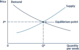
Marshall believed that demand and supply together determine the equilibrium price (P * ) and quantity (Q * ) of a good. The positive slope of the supply curve reflects diminishing returns (increasing marginal cost), whereas the negative slope of the demand curve reflects diminishing marginal usefulness. P * is an equilibrium price. Any other price results in either a surplus or a shortage.