Introductory Econometrics: A Modern Approach 6th Edition by Jeffrey M Wooldridge

Exercise 5

Use the data in WAGEPRC.RAW for this exercise. Problem 11.5 gave estimates of a finite distributed lag model of gprice on gwage, where 12 lags of gwage are used.

(i) Estimate a simple geometric DL model of gprice on gwage. In particular, estimate equation by OLS. What are the estimated impact propensity and LRP? Sketch the estimated lag distribution.

(ii) Compare the estimated IP and LRP to those obtained in Problem. How do the estimated lag distributions compare?

(iii) Now, estimate the rational distributed lag model from (18.16). Sketch the lag distribution and compare the estimated IP and LRP to those obtained in part (ii).

For the U.S. economy, let gprice denote the monthly growth in the overall price level and let gwage be the monthly growth in hourly wages. [These are both obtained as differences of logarithms: gprice log(price) and gwage log(wage).] Using the monthly data in WAGEPRC.RAW, we estimate the following distributed lag model:

Problem

(i) Sketch the estimated lag distribution. At what lag is the effect of gwage on gprice largest? Which lag has the smallest coefficient?

(ii) For which lags are the t statistics less than two?

(iii) What is the estimated long-run propensity? Is it much different than one? Explain

what the LRP tells us in this example.

(iv) What regression would you run to obtain the standard error of the LRP directly?

(v) How would you test the joint significance of six more lags of gwage? What would be the dfs in the F distribution? (Be careful here; you lose six more observations.)

Equation

Step 1 of 4

(i)

Estimating the simple geometric DL model of on, the result is:

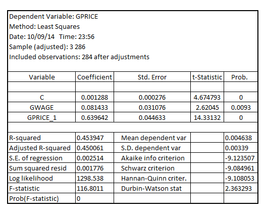
The Impact propensity is given by the coefficient of which is 0.081433

The LRP is given by:

The estimated lag distribution is given by:

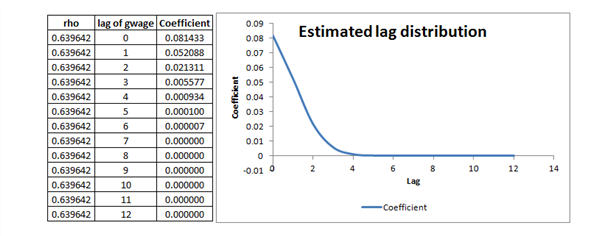
At a lag of “j” of gwage, the coefficient of gwage is given by