expand icon
book Introductory Econometrics: A Modern Approach 6th Edition by Jeffrey M Wooldridge cover

Introductory Econometrics: A Modern Approach 6th Edition by Jeffrey M Wooldridge

Edition 6ISBN: 130527010X
book Introductory Econometrics: A Modern Approach 6th Edition by Jeffrey M Wooldridge cover

Introductory Econometrics: A Modern Approach 6th Edition by Jeffrey M Wooldridge

Edition 6ISBN: 130527010X
Exercise 19

A common method for estimating Engel curves is to model expenditure shares as a function of total expenditure, and possibly demographic variables. A common specification has the form

 A common method for estimating <i>Engel curves </i>is to model expenditure shares as a function of total expenditure, and possibly demographic variables. A common specification has the form   where <i>sgood </i>is the fraction of spending on a particular good out of total expenditure and <i>ltotexpend </i>is the log of total expenditure. The sign and magnitude of <i>   </i>are of interest across various expenditure categories. To account for the potential endogeneity of <i>ltotexpend—</i>which can be viewed as an omitted variables or simultaneous equations problem, or both—the log of family income is often used as an instrumental variable. Let <i>lincome </i>denote the log of family income. For the remainder of this question, use the data in EXPENDSHARE.RAW, which comes from Blundell, Duncan, and Pendakur (1998). (i) Use <i>sfood</i>, the share of spending on food, as the dependent variable. What is the range of values of <i>sfood</i>? Are you surprised there are no zeros? (ii) Estimate the equation <i>   </i> by OLS, and report the coefficient on <i>ltotexpend</i>, <i>   </i>along with its heteroskedasticity- robust standard error. Intepret the result. (iii) Using <i>lincome </i>as an IV for <i>ltotexpend</i>, estimate the reduced form equation for <i>ltotexpend</i>; be sure to include <i>age </i>and <i>kids</i>. Assuming <i>lincome </i>is exogenous in (16.43), is <i>lincome </i>a valid IV for <i>ltotexpend</i>? (iv) Now estimate (16.43) by instrumental variables. How does <i>   </i>compare with <i>   </i>What about the robust 95% confidence intervals? (v) Use the test in Section 15.5 to test the null hypothesis that <i>ltotexpend </i>is exogenous in (16.43). Be sure to report and interpret the <i>p</i>-value. Are there any overidentifying restrictions to test? (vi) Substitute <i>salcohol </i>for <i>sfood </i>in (16.43) and estimate the equation by OLS and 2SLS. Now what do you find for the coefficients on <i>ltotexpend</i>?

where sgood is the fraction of spending on a particular good out of total expenditure and ltotexpend is the log of total expenditure. The sign and magnitude of  A common method for estimating <i>Engel curves </i>is to model expenditure shares as a function of total expenditure, and possibly demographic variables. A common specification has the form   where <i>sgood </i>is the fraction of spending on a particular good out of total expenditure and <i>ltotexpend </i>is the log of total expenditure. The sign and magnitude of <i>   </i>are of interest across various expenditure categories. To account for the potential endogeneity of <i>ltotexpend—</i>which can be viewed as an omitted variables or simultaneous equations problem, or both—the log of family income is often used as an instrumental variable. Let <i>lincome </i>denote the log of family income. For the remainder of this question, use the data in EXPENDSHARE.RAW, which comes from Blundell, Duncan, and Pendakur (1998). (i) Use <i>sfood</i>, the share of spending on food, as the dependent variable. What is the range of values of <i>sfood</i>? Are you surprised there are no zeros? (ii) Estimate the equation <i>   </i> by OLS, and report the coefficient on <i>ltotexpend</i>, <i>   </i>along with its heteroskedasticity- robust standard error. Intepret the result. (iii) Using <i>lincome </i>as an IV for <i>ltotexpend</i>, estimate the reduced form equation for <i>ltotexpend</i>; be sure to include <i>age </i>and <i>kids</i>. Assuming <i>lincome </i>is exogenous in (16.43), is <i>lincome </i>a valid IV for <i>ltotexpend</i>? (iv) Now estimate (16.43) by instrumental variables. How does <i>   </i>compare with <i>   </i>What about the robust 95% confidence intervals? (v) Use the test in Section 15.5 to test the null hypothesis that <i>ltotexpend </i>is exogenous in (16.43). Be sure to report and interpret the <i>p</i>-value. Are there any overidentifying restrictions to test? (vi) Substitute <i>salcohol </i>for <i>sfood </i>in (16.43) and estimate the equation by OLS and 2SLS. Now what do you find for the coefficients on <i>ltotexpend</i>? are of interest across various expenditure categories. To account for the potential endogeneity of ltotexpend—which can be viewed as an omitted variables or simultaneous equations problem, or both—the log of family income is often used as an instrumental variable. Let lincome denote the log of family income. For the remainder of this question, use the data in EXPENDSHARE.RAW, which comes from Blundell, Duncan, and Pendakur (1998).

(i) Use sfood, the share of spending on food, as the dependent variable. What is the range of values of sfood? Are you surprised there are no zeros?

(ii) Estimate the equation

 A common method for estimating <i>Engel curves </i>is to model expenditure shares as a function of total expenditure, and possibly demographic variables. A common specification has the form   where <i>sgood </i>is the fraction of spending on a particular good out of total expenditure and <i>ltotexpend </i>is the log of total expenditure. The sign and magnitude of <i>   </i>are of interest across various expenditure categories. To account for the potential endogeneity of <i>ltotexpend—</i>which can be viewed as an omitted variables or simultaneous equations problem, or both—the log of family income is often used as an instrumental variable. Let <i>lincome </i>denote the log of family income. For the remainder of this question, use the data in EXPENDSHARE.RAW, which comes from Blundell, Duncan, and Pendakur (1998). (i) Use <i>sfood</i>, the share of spending on food, as the dependent variable. What is the range of values of <i>sfood</i>? Are you surprised there are no zeros? (ii) Estimate the equation <i>   </i> by OLS, and report the coefficient on <i>ltotexpend</i>, <i>   </i>along with its heteroskedasticity- robust standard error. Intepret the result. (iii) Using <i>lincome </i>as an IV for <i>ltotexpend</i>, estimate the reduced form equation for <i>ltotexpend</i>; be sure to include <i>age </i>and <i>kids</i>. Assuming <i>lincome </i>is exogenous in (16.43), is <i>lincome </i>a valid IV for <i>ltotexpend</i>? (iv) Now estimate (16.43) by instrumental variables. How does <i>   </i>compare with <i>   </i>What about the robust 95% confidence intervals? (v) Use the test in Section 15.5 to test the null hypothesis that <i>ltotexpend </i>is exogenous in (16.43). Be sure to report and interpret the <i>p</i>-value. Are there any overidentifying restrictions to test? (vi) Substitute <i>salcohol </i>for <i>sfood </i>in (16.43) and estimate the equation by OLS and 2SLS. Now what do you find for the coefficients on <i>ltotexpend</i>?

by OLS, and report the coefficient on ltotexpend,  A common method for estimating <i>Engel curves </i>is to model expenditure shares as a function of total expenditure, and possibly demographic variables. A common specification has the form   where <i>sgood </i>is the fraction of spending on a particular good out of total expenditure and <i>ltotexpend </i>is the log of total expenditure. The sign and magnitude of <i>   </i>are of interest across various expenditure categories. To account for the potential endogeneity of <i>ltotexpend—</i>which can be viewed as an omitted variables or simultaneous equations problem, or both—the log of family income is often used as an instrumental variable. Let <i>lincome </i>denote the log of family income. For the remainder of this question, use the data in EXPENDSHARE.RAW, which comes from Blundell, Duncan, and Pendakur (1998). (i) Use <i>sfood</i>, the share of spending on food, as the dependent variable. What is the range of values of <i>sfood</i>? Are you surprised there are no zeros? (ii) Estimate the equation <i>   </i> by OLS, and report the coefficient on <i>ltotexpend</i>, <i>   </i>along with its heteroskedasticity- robust standard error. Intepret the result. (iii) Using <i>lincome </i>as an IV for <i>ltotexpend</i>, estimate the reduced form equation for <i>ltotexpend</i>; be sure to include <i>age </i>and <i>kids</i>. Assuming <i>lincome </i>is exogenous in (16.43), is <i>lincome </i>a valid IV for <i>ltotexpend</i>? (iv) Now estimate (16.43) by instrumental variables. How does <i>   </i>compare with <i>   </i>What about the robust 95% confidence intervals? (v) Use the test in Section 15.5 to test the null hypothesis that <i>ltotexpend </i>is exogenous in (16.43). Be sure to report and interpret the <i>p</i>-value. Are there any overidentifying restrictions to test? (vi) Substitute <i>salcohol </i>for <i>sfood </i>in (16.43) and estimate the equation by OLS and 2SLS. Now what do you find for the coefficients on <i>ltotexpend</i>? along with its heteroskedasticity- robust standard error. Intepret the result.

(iii) Using lincome as an IV for ltotexpend, estimate the reduced form equation for ltotexpend; be sure to include age and kids. Assuming lincome is exogenous in (16.43), is lincome a valid IV for ltotexpend?

(iv) Now estimate (16.43) by instrumental variables. How does  A common method for estimating <i>Engel curves </i>is to model expenditure shares as a function of total expenditure, and possibly demographic variables. A common specification has the form   where <i>sgood </i>is the fraction of spending on a particular good out of total expenditure and <i>ltotexpend </i>is the log of total expenditure. The sign and magnitude of <i>   </i>are of interest across various expenditure categories. To account for the potential endogeneity of <i>ltotexpend—</i>which can be viewed as an omitted variables or simultaneous equations problem, or both—the log of family income is often used as an instrumental variable. Let <i>lincome </i>denote the log of family income. For the remainder of this question, use the data in EXPENDSHARE.RAW, which comes from Blundell, Duncan, and Pendakur (1998). (i) Use <i>sfood</i>, the share of spending on food, as the dependent variable. What is the range of values of <i>sfood</i>? Are you surprised there are no zeros? (ii) Estimate the equation <i>   </i> by OLS, and report the coefficient on <i>ltotexpend</i>, <i>   </i>along with its heteroskedasticity- robust standard error. Intepret the result. (iii) Using <i>lincome </i>as an IV for <i>ltotexpend</i>, estimate the reduced form equation for <i>ltotexpend</i>; be sure to include <i>age </i>and <i>kids</i>. Assuming <i>lincome </i>is exogenous in (16.43), is <i>lincome </i>a valid IV for <i>ltotexpend</i>? (iv) Now estimate (16.43) by instrumental variables. How does <i>   </i>compare with <i>   </i>What about the robust 95% confidence intervals? (v) Use the test in Section 15.5 to test the null hypothesis that <i>ltotexpend </i>is exogenous in (16.43). Be sure to report and interpret the <i>p</i>-value. Are there any overidentifying restrictions to test? (vi) Substitute <i>salcohol </i>for <i>sfood </i>in (16.43) and estimate the equation by OLS and 2SLS. Now what do you find for the coefficients on <i>ltotexpend</i>? compare with  A common method for estimating <i>Engel curves </i>is to model expenditure shares as a function of total expenditure, and possibly demographic variables. A common specification has the form   where <i>sgood </i>is the fraction of spending on a particular good out of total expenditure and <i>ltotexpend </i>is the log of total expenditure. The sign and magnitude of <i>   </i>are of interest across various expenditure categories. To account for the potential endogeneity of <i>ltotexpend—</i>which can be viewed as an omitted variables or simultaneous equations problem, or both—the log of family income is often used as an instrumental variable. Let <i>lincome </i>denote the log of family income. For the remainder of this question, use the data in EXPENDSHARE.RAW, which comes from Blundell, Duncan, and Pendakur (1998). (i) Use <i>sfood</i>, the share of spending on food, as the dependent variable. What is the range of values of <i>sfood</i>? Are you surprised there are no zeros? (ii) Estimate the equation <i>   </i> by OLS, and report the coefficient on <i>ltotexpend</i>, <i>   </i>along with its heteroskedasticity- robust standard error. Intepret the result. (iii) Using <i>lincome </i>as an IV for <i>ltotexpend</i>, estimate the reduced form equation for <i>ltotexpend</i>; be sure to include <i>age </i>and <i>kids</i>. Assuming <i>lincome </i>is exogenous in (16.43), is <i>lincome </i>a valid IV for <i>ltotexpend</i>? (iv) Now estimate (16.43) by instrumental variables. How does <i>   </i>compare with <i>   </i>What about the robust 95% confidence intervals? (v) Use the test in Section 15.5 to test the null hypothesis that <i>ltotexpend </i>is exogenous in (16.43). Be sure to report and interpret the <i>p</i>-value. Are there any overidentifying restrictions to test? (vi) Substitute <i>salcohol </i>for <i>sfood </i>in (16.43) and estimate the equation by OLS and 2SLS. Now what do you find for the coefficients on <i>ltotexpend</i>? What about the robust 95% confidence intervals?

(v) Use the test in Section 15.5 to test the null hypothesis that ltotexpend is exogenous in (16.43). Be sure to report and interpret the p-value. Are there any overidentifying restrictions to test?

(vi) Substitute salcohol for sfood in (16.43) and estimate the equation by OLS and 2SLS. Now what do you find for the coefficients on ltotexpend?

Step-by-step solution
Verified
like image
like image

Step 1 of 10

(i)

Consider the provided data of EXPENDSHARES and calculate the minimum and maximum values in Excel as shown below:

    <div class=answer> (i) Consider the provided data of EXPENDSHARES and calculate the minimum and maximum values in Excel as shown below:     Therefore, the range of values for <i>sfood </i>is 0.0571 to 0.789. The logical range for <i>sfood </i>is from 0 to 1 but it is not surprising to get no zeros because every individual needs to invest some amount on food.

    <div class=answer> (i) Consider the provided data of EXPENDSHARES and calculate the minimum and maximum values in Excel as shown below:     Therefore, the range of values for <i>sfood </i>is 0.0571 to 0.789. The logical range for <i>sfood </i>is from 0 to 1 but it is not surprising to get no zeros because every individual needs to invest some amount on food.

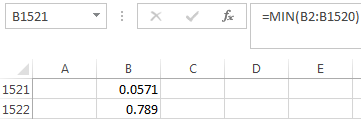
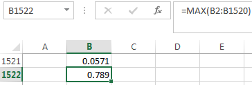
Therefore, the range of values for sfood is 0.0571 to 0.789. The logical range for sfood is from 0 to 1 but it is not surprising to get no zeros because every individual needs to invest some amount on food.


Step 2 of 10


Step 3 of 10


Step 4 of 10


Step 5 of 10


Step 6 of 10


Step 7 of 10


Step 8 of 10


Step 9 of 10


Step 10 of 10

close menu
Introductory Econometrics: A Modern Approach 6th Edition by Jeffrey M Wooldridge
cross icon