Introductory Econometrics: A Modern Approach 6th Edition by Jeffrey M Wooldridge

Exercise 20

The data set DRIVING.RAW includes state-level panel data (for the 48 continental U.S. states) from 1980through 2004, for a total of 25 years. Various driving laws are indicated in the data set, including the alcohol level at which drivers are considered legally intoxicated. There are also indicators for “per se” laws where licenses can be revoked without a trial—and seat belt laws. Some economics and demographic variables are also included.

(i) How is the variable totfatrte defined? What is the average of this variable in the years 1980, 1992, and 2004? Run a regression of totfatrte on dummy variables for the years 1981 through 2004, and describe what you find. Did driving become safer over this period? Explain.

(ii) Add the variables bac08, bac10, perse, sbprim, sbsecon, sl70plus, gdl, perc14_24, unem, and vehicmilespc to the regression from part (i). Interpret the coefficients on bac8 and bac10. Do per se laws have a negative effect on the fatality rate? What about having a primary seat belt law? (Note that if a law was enacted sometime within a year the fraction of the year is recorded in place of the zero-one indicator.)

(iii) Reestimate the model from part (ii) using fixed effects (at the state level). How do the coefficients on bac08, bac10, perse, and sbprim compare with the pooled OLS estimates? Which set of estimates do you think is more reliable?

(iv) Suppose that vehicmilespc, the number of miles driven per capita, increases by 1,000. Using the FE estimates, what is the estimated effect on totfatrte? Be sure to interpret the estimate as if explaining to a layperson.

(v) If there is serial correlation or heteroskedasticity in the idiosyncratic errors of the model then the standard errors in part (iii) are invalid. If possible, use “cluster” robust standard errors for the fixed effects estimates. What happens to the statistical significance of the policy variables in part (iii)?

Step 1 of 10

(i)

The variable is total fatalities per 100,000 populations

The average of in 1980, 1992 and 2004 are 25.494, 17.157 and 16.728 respectively

Estimating the regression of on dummy variables for the year 1981 to 2004, the result is:

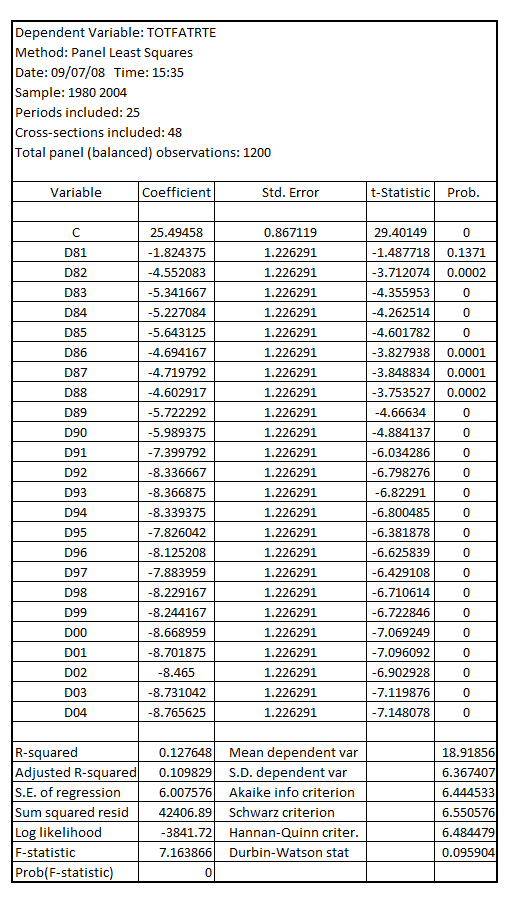
It is observed that the coefficients of the year dummy variables except for 1981 are individually significant at 5% level of significance as their respective p-value is less than the critical p-value of 0.05 at 5% level of significance

It is also observed that the coefficients of the year dummy variables for the years 1981 to 2004 are negative, indicating that the total fatalities per 100,000 populations is negatively related to years, indicating that the driving became safer over this period