Introductory Econometrics: A Modern Approach 6th Edition by Jeffrey M Wooldridge

Exercise 15

Use the data in MATHPNL.RAW for this exercise. You will do a fixed effects version of the first differencing done in Computer Exercise The model of interest is

where the first available year (the base year) is 1993 because of the lagged spending variable.

(i) Estimate the model by pooled OLS and report the usual standard errors. You should include an intercept along with the year dummies to allow a to have a nonzero expected value. What are the estimated effects of the spending variables? Obtain the OLS residuals, .

(ii) Is the sign of the lunch t coefficient what you expected? Interpret the magnitude of the coefficient. Would you say that the district poverty rate has a big effect on test pass rates?

(iii) Compute a test for AR(1) serial correlation using the regression You should use the years 1994 through 1998 in the regression. Verify that there is strong positive serial correlation and discuss why.

(iv) Now, estimate the equation by fixed effects. Is the lagged spending variable still significant?

(v) Why do you think, in the fixed effects estimation, the enrollment and lunch program variables are jointly insignificant?

(vi) Define the total, or long-run, effect of spending as ?1 = ?1 + ?2. Use the substitution ?1 = ?1- ?2 to obtain a standard error for 01. [Hint: Standard fixed effects estimation using as explanatory variables should do it.]

The file MATHPNL.RAW contains panel data on school districts in Michigan for the years 1992 through 1998. It is the district-level analogue of the school-level data used by Papke (2005). The response variable of interest in this question is math4, the percentage of fourth graders in a district receiving a passing score on a standardized math test. The key explanatory variable is rexpp, which is real expenditures per pupil in the district. The amounts are in 1997 dollars. The spending variable will appear in logarithmic form.

(i) Consider the static unobserved effects model

where enrolit is total district enrollment and lunchit is the percentage of students in the district eligible for the school lunch program. (So lunchit is a pretty good measure of the district-wide poverty rate.) Argue that _1/10 is the percentage point change in math4it when real per-student spending increases by roughly 10%.

(ii) Use first differencing to estimate the model in part (i). The simplest approach is to allow an intercept in the first-differenced equation and to include dummy variables for the years 1994 through 1998. Interpret the coefficient on the spending variable.

(iii) Now, add one lag of the spending variable to the model and reestimate using first differencing. Note that you lose another year of data, so you are only using changes starting in 1994. Discuss the coefficients and significance on the current and lagged spending variables.

(iv) Obtain heteroskedasticity-robust standard errors for the first-differenced regression in part (iii). How do these standard errors compare with those from part (iii) for the spending variables?

(v) Now, obtain standard errors robust to both heteroskedasticity and serial correlation.

What does this do to the significance of the lagged spending variable?

(vi) Verify that the differenced errors rit ?uit have negative serial correlation by carrying out a test of AR(1) serial correlation.

(vii) Based on a fully robust joint test, does it appear necessary to include the enrollment and lunch variables in the model?

Step 1 of 8

(i)

Estimating the model using pooled OLS, the result is:

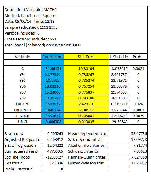
The usual standard errors of the coefficients of the respective explanatory variables included in the model are highlighted in “Yellow”

The coefficients of the spending variable andare 0.533937 and 9.049174 respectively

The OLS residuals is obtained by subtracting estimated from actual

The estimated is obtained by the model