Introductory Econometrics: A Modern Approach 6th Edition by Jeffrey M Wooldridge

Exercise 12

Let hy6t denote the three-month holding yield (in percent) from buying a six-month T-bill at time (t – 1) and selling it at time t (three months hence) as a three-month

T-bill. Let hy3t-1 be the three-month holding yield from buying a three-month T-bill at time (t – 1). At time (t – 1), hy3t-1 is known, whereas hy6t is unknown because p3t (the price of three-month T-bills) is unknown at time (t – 1). The expectations hypothesis (EH) says that these two different three-month investments should be the

same, on average. Mathematically, we can write this as a conditional expectation:

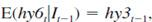
where It-1 denotes all observable information up through time t – 1. This suggests estimating the model 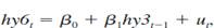and testing H0: ? = 1. (We can also test H0: ?0 = 0, but we often allow for a term premium for buying assets with different maturities, so that ?0 ? 0.)

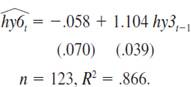
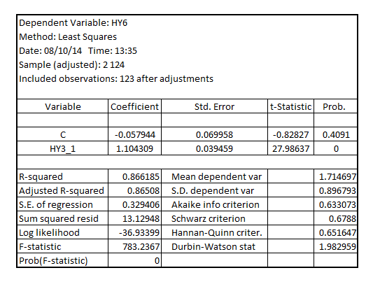
(i) Estimating the previous equation by OLS using the data in INTQRT.RAW (spaced every three months) gives

Do you reject H0: ?1=1 against H0:? 1 ? 1 at the 1% significance level? Does the estimate seem practically different from one?

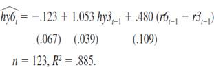
(ii) Another implication of the EH is that no other variables dated as t - 1 or earlier should help explain hy6t, once hy3t-1 has been controlled for. Including one lag of the spread between six-month and three-month T-bill rates gives

Now, is the coefficient on hy3t - 1 statistically different from one? Is the lagged spread term significant? According to this equation, if, at time t - 1, r6 is above r3, should you invest in six-month or three-month T-bills?

(iii) The sample correlation between hy3t and hy3t - 1 is .914. Why might this raise some concerns with the previous analysis?

(iv) How would you test for seasonality in the equation estimated in part (ii)?

Step 1 of 8

Consider to be three month holding yield (in percent) from buying six month T-bill at time and selling it at as the three month T-bill.

Consider to be three month holding yield from buying a three-month T-bill at time .

The regression model is

The result is:

The standard form of the model is