Introductory Econometrics: A Modern Approach 6th Edition by Jeffrey M Wooldridge

Exercise 9

Use the data in PNTSPRD.RAW for this exercise.

(i) The variable sprdcvr is a binary variable equal to one if the Las Vegas point spread for a college basketball game was covered. The expected value of sprdcvr, say 1, is the probability that the spread is covered in a randomly selected game. Test H0: µ = .5 against H1: µ ? .5 at the 10% significance level and discuss your findings. (Hint: This is easily done using a t test by regressing sprdcvr on an intercept only.)

(ii) How many games in the sample of 553 were played on a neutral court?

(iii) Estimate the linear probability model

and report the results in the usual form. (Report the usual OLS standard errors and the heteroskedasticity-robust standard errors.) Which variable is most significant, both practically and statistically?

(iv) Explain why, under the null hypothesis H0: ?1 = ?2 = ?3 = ?4 = 0, there is no heteroskedasticity in the model.

(v) Use the usual F statistic to test the hypothesis in part (iv). What do you conclude?

(vi) Given the previous analysis, would you say that it is possible to systematically predict whether the Las Vegas spread will be covered using information available prior to the game?

Step 1 of 9

(i)

Given that the variable is the binary variable equal to 1 if Las Vegas point spread for the college basket game was covered.

It shall be noted that the expected value ofis, which is the probability that the spread is covered in a randomly selected game.

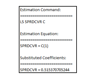
Regressingon the intercept only, the result is:

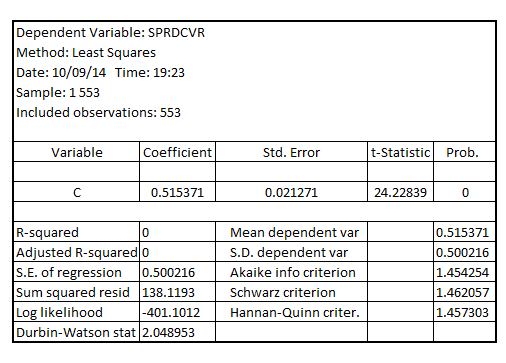
Now testing for the expected value of which is given by the coefficient of intercept being equal to 0.5 at 10% level of significance using the Wald test, the result is:

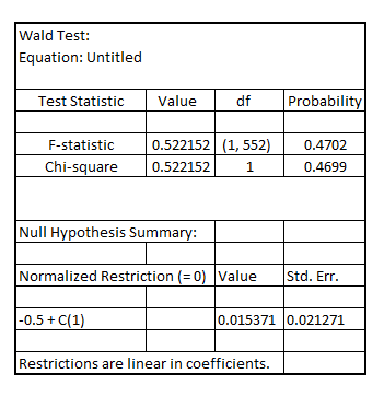
Since, the p-value of F-statistic is 0.4702 which is greater than the critical p-value of 0.1 at 10% level of significance, it is indicative that there is no statistically significant difference of expected value of from 0.5 at 10% level of significance