
Introductory Econometrics: A Modern Approach 6th Edition by Jeffrey M Wooldridge
Edition 6ISBN: 130527010XIntroductory Econometrics: A Modern Approach 6th Edition by Jeffrey M Wooldridge
Edition 6ISBN: 130527010XUse the data in HTV.RAW to answer this question. See also Computer Exercise C10 in Chapter 3.
(i) Estimate the regression model

by OLS and report the results in the usual form. Test the null hypothesis that educ is linearly related to abil against the alternative that the relationship is quadratic.
(ii) Using the equation in part (i), test  against a two-sided alternative. What is the p-value of the test?
(iii) Add the two college tuition variables to the regression from part (i) and determine whether they are jointly statistically significant.
(iv) What is the correlation between tuit17 and tuit18? Explain why using the average of the tuition over the two years might be preferred to adding each separately. What happens when you do use the average?
(v) Do the findings for the average tuition variable in part (iv) make sense when interpreted causally? What might be going on?
Reference: Excercise C10:
Use the data in HTV.RAW to answer this question. The data set includes information on wages, education, parents’ education, and several other variables for 1,230 working men in 1991.
(i) What is the range of the educ variable in the sample? What percentage of men completed 12th grade but no higher grade? Do the men or their parents have, on average, higher levels of education?
(ii) Estimate the regression model
by OLS and report the results in the usual form. How much sample variation in educ is explained by parents’ education? Interpret the coefficient on motheduc.
(iii) Add the variable abil (a measure of cognitive ability) to the regression from part (ii), and report the results in equation form. Does “ability” help to explainvariations in education, even after controlling for parents’ education? Explain.
(iv) (Requires calculus) Now estimate an equation where abil appears in quadratic form:

Using the estimates  use calculus to find the value of abil, call it abil*, where educ is minimized. (The other coefficients and values of parents’ education variables have no effect; we are holding parents’ education fixed.) Notice that abil is measured so that negative values are permissible. You might also verify that the second derivative is positive so that you do indeed have a minimum.
(v) Argue that only a small fraction of men in the sample have “ability” less than the value calculated in part (iv). Why is this important?
(vi) If you have access to a statistical program that includes graphing capabilities, use the estimates in part (iv) to graph the relationship beween the predicted education and abil. Let motheduc and fatheduc have their average values in the sample, 12.18 and 12.45, respectively.
Step 1 of 7
(i)
Estimating the regression model given by:

The result is:
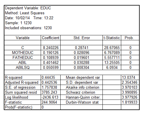
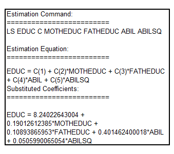
The equation form of the model is given by:

Testing the null hypothesis that is linearly related to
  against the alternative that the relationship is quadratic using Wald test, the result is:

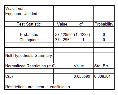
It shall be observed that the p-value of F-statistic is 0.0000 which is less than the critical p-value of 0.05 at 5% level of significance indicating that the null hypothesis that  is linearly related to
  is rejected. Hence, it can be inferred that the relationship between
  and
and is quadratic
Step 2 of 7
Step 3 of 7
Step 4 of 7
Step 5 of 7
Step 6 of 7
Step 7 of 7
Why don’t you like this exercise?
Other


