
Introductory Econometrics: A Modern Approach 6th Edition by Jeffrey M Wooldridge
Edition 6ISBN: 130527010XIntroductory Econometrics: A Modern Approach 6th Edition by Jeffrey M Wooldridge
Edition 6ISBN: 130527010XUse the data in ELEM94_95 to answer this question. The findings can be compared with those in Table 4.1. The dependent variable lavgsal is the log of average teacher salary and bs is the ratio of average benefits to average salary (by school).
(i) Run the simple regression of lavgsal on bs. Is the estimated slope statistically different from zero? Is it statistically different from — 1?
(ii) Add the variables lenrol and lstaff to the regression from part (i). What happens to the coefficient on bs? How does the situation compare with that in Table 4.1?
(iii) How come the standard error on the bs coefficient is smaller in part (ii) than in part (i)? (Hint: What happens to the error variance versus multicollinearity when lenrol and lstaff are added?)
(iv) How come the coefficient on lstaff is negative? Is it large in magnitude?
(v) Now add the variable lunch to the regression. Holding other factors fixed, are teachers being compensated for teaching students from disadvantaged backgrounds? Explain.
(vi) Overall, is the pattern of results that you find with ELEM94_95.RAW consistent with the pattern in Table 4.1?
Step 1 of 9
(i)
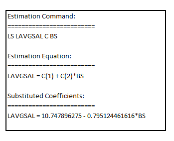
Estimating the simple regression of  on
on , the result is:

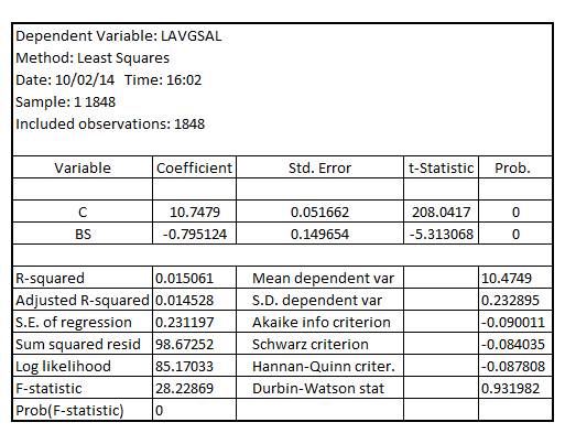
Testing for the estimated slope being statistically significantly different from zero using Wald test, the result is:

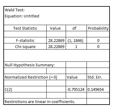
Since, the p-value of F-statistic is 0.0000 which is less than the critical p-value of 0.05 at 5% level of significance, it is inferred that the estimated slope is statistically significant at 5% level of significance
Testing for the estimated slope being statistically significantly different from -1 using Wald test, the result is:

Step 2 of 9
Step 3 of 9
Step 4 of 9
Step 5 of 9
Step 6 of 9
Step 7 of 9
Step 8 of 9
Step 9 of 9
Why don’t you like this exercise?
Other


