Deck 8: Combining Forecast Results
Full screen (f)
Question
Question
Question
Question
Question
Question
Air Carrier Traffic Statistics Monthly is a handbook of airline data published by the U.S. Department of Transportation. In this book you will find revenue passenger-miles (RPM) traveled on major airlines on international flights. Airlines regularly try to predict accurately the RPM for future periods; this gives the airline a picture of what equipment needs might be and is helpful in keeping costs at a minimum.
The revenue passenger-miles for international flights on major international airlines is shown in the accompanying table for the period Jan-1979 to Feb-1984. Also shown is personal income during the same period, in billions of dollars.
a. Build a multiple-regression model for the data to predict RPM for the next month. Check the data for any trend, and be careful to account for any seasonality. You should easily be able to obtain a forecast model with an R -squared of about 0.70 that exhibits little serial correlation.
b. Use the same data to compute a time-series decomposition model, and again forecast for one month in the future.
c. Judging from the root-mean-squared error, which of the models in parts ( a ) and ( b ) proved to be the best forecasting model? Now combine the two models, using weighting scheme like that shown in Table 8.1. Choose various weights until you believe you have come close to the optimum weighting scheme. Does this combined model perform better (according to RMSE) than either of the two original models? Why do you believe the combined model behaves in this way?
d. Try one other forecasting method of your choice on these data, and combine the results with the multiple-regression model. Do you obtain a better forecast (according to RMSE) than with either of your two original models?
Question
Estimating the volume of loans that will be made at a credit union is crucial to effective cash management in those institutions. In the table that follows are quarterly data for a real credit union located in a midwestern city. Credit unions are financial institutions similar to banks, but credit unions are not-for-profit firms whose members are the actual owners (remember their slogan, "It's where you belong"). The members may be both depositors in and borrowers from the credit union.
 a. Estimate a multiple-regression model to estimate loan demand and calculate its root-mean- squared error.
b. Estimate a time-series decomposition model to estimate loan demand with the same data and calculate its root-mean-squared error.
c. Combine the models in parts ( a ) and ( b ) and determine whether the combined model performs better than either or both of the original models. Try to explain why you obtained the results you did.
a. Estimate a multiple-regression model to estimate loan demand and calculate its root-mean- squared error.b. Estimate a time-series decomposition model to estimate loan demand with the same data and calculate its root-mean-squared error.
c. Combine the models in parts ( a ) and ( b ) and determine whether the combined model performs better than either or both of the original models. Try to explain why you obtained the results you did.
Question
HeathCo Industries, a producer of a line of skiwear, has been the subject of exercises in several earlier chapters of the text. The data for its sales and two potential causal variables, income (INCOME) and the northern-region unemployment rate (NRUR), are repeated in the following table:
 a. Develop a multiple-regression model of SALES as a function of both INCOME and NRUR:
SALES = a + b 1 (INCOME) + b 2 (NRUR)
Use this model to forecast sales for 2008Q1-2008Q4 (call your regression forecast series SFR), given that INCOME and NRUR for 2004 have been forecast to be:
 b. Calculate the RMSE for your regression model for both the historical period (1998Q1-2007Q4) and the forecast horizon (2008Q1-2008Q4).
 d. Solely on the basis of the historical data, which model appears to be the best? Why?
e. Now prepare a combined forecast (SCF) using the regression technique described in this chapter. In the standard regression:
SALES = a + b 1 (SFR) + b 2 (SFW)
Is the intercept essentially zero? Why? If it is, do the following regression as a basis
for developing SCF:
SALES = b 1 (SFR) + b 2 (SFW)
Given the historical RMSEs found in parts ( b ) and ( c ), do the values for b 1 and b 2 seem plausible? Explain.
f. Calculate the RMSEs for SCF:
 Did combining models reduce the RMSE in the historical period? What about the actual forecast?
a. Develop a multiple-regression model of SALES as a function of both INCOME and NRUR:SALES = a + b 1 (INCOME) + b 2 (NRUR)
Use this model to forecast sales for 2008Q1-2008Q4 (call your regression forecast series SFR), given that INCOME and NRUR for 2004 have been forecast to be:
b. Calculate the RMSE for your regression model for both the historical period (1998Q1-2007Q4) and the forecast horizon (2008Q1-2008Q4). d. Solely on the basis of the historical data, which model appears to be the best? Why?e. Now prepare a combined forecast (SCF) using the regression technique described in this chapter. In the standard regression:
SALES = a + b 1 (SFR) + b 2 (SFW)
Is the intercept essentially zero? Why? If it is, do the following regression as a basis
for developing SCF:
SALES = b 1 (SFR) + b 2 (SFW)
Given the historical RMSEs found in parts ( b ) and ( c ), do the values for b 1 and b 2 seem plausible? Explain.
f. Calculate the RMSEs for SCF:
Did combining models reduce the RMSE in the historical period? What about the actual forecast? Question
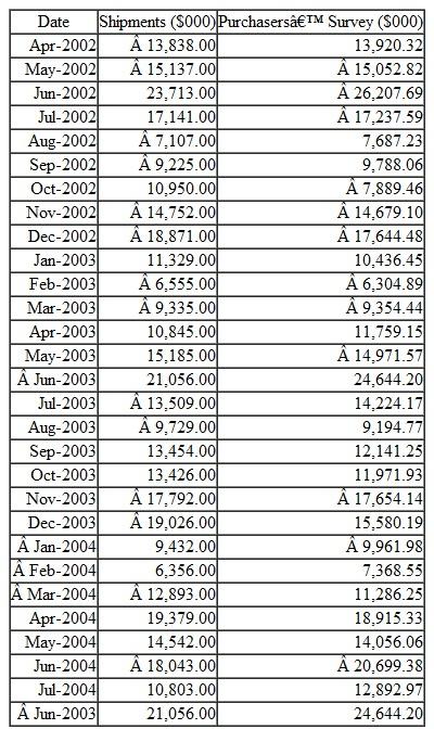
Your company produces a favorite summertime food product, and you have been placed in charge of forecasting shipments of this product. The historical data below represent your company's past experience with the product.
a. Since the data appear to have both seasonality and trend, you should estimate a Winters' model and calculate its root-mean-squared error.
b. You also have access to a survey of the potential purchasers of your product. This information has been collected for some time, and it has proved to be quite accurate for predicting shipments in the past. Calculate the root-mean-squared error of the purchasers' survey data.
c. After checking for bias, combine the forecasts in parts ( a ) and ( b ) and determine if a combined model may forecast better than either single model.

Unlock Deck
Sign up to unlock the cards in this deck!
Unlock Deck
Unlock Deck
1/9
Play
Full screen (f)
Deck 8: Combining Forecast Results
1
Assume you would like to use a Winters' model and combine the forecast results with a multiple-regression model. Use the regression technique to decide on the weighting to attach to each forecast.
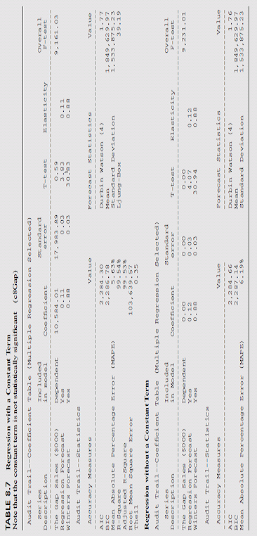
To see if both models may reasonably be used in a combined forecast, run the regression that uses The Gap sales as the dependent variable and the two forecasts (one from the Winters' model and the other from the multiple-regression model) as the explanatory variables. The regression (shown in upper half of Table 8.7) indicates that there is little significance attached to the constant term (because of its t -statistic of 1.08), and so we may reasonably attempt to combine the models.
2
Explain why a combined model might be better than any of the original contributing models. Could there be cases in which a combined model would show no gain in forecast accuracy over the original models? Give an example where this situation might be likely to occur.
One recent and popular strategy in forecasting is to use combination of the output from different forecasting systems. Few researchers have established with evidences that combined models often predict forecasts with higher accuracy.
A combined model might be better than an individual forecasting model due to the following two basic reasons:
o Generally, a model is discarded based on the poor fit and accuracy of the output. But it has to be remembered that some variables included in a discarded model may not be available in the best (i.e. most accurate) model. So, excluding one or more such variables are lost opportunities.
o The discarded method of forecasting may actually use some relationships among the variables which may be not there in the best model. This is also an opportunity loss.
When the combined model is used, it tries to minimize all these opportunity losses by combining several methods of forecasts. Therefore, a combined model may lead to a forecast which is more accurate than any individual model.
However, a combined model may not always guarantee to yield a forecast with higher gains compared to individual forecasts. As described above, if different method does not include new variables or new relationships, it is primarily useless to utilize them in combined forecast.
For example, two individual method of forecasting trend can be linear regression and central moving average. Note that in both the case, neither different variables are getting used not new relationships are levered. So, in this case combining these two methods will not lead to any better forecast than to use best (most accurate) of them.
3
Combine the two methods (i.e., the Winters' and the multiple-regression models) with the calculated weighting scheme, and construct a combined forecast model.
The two models are combined by running the same regression through the origin (shown in the lower half of Table 8.7). Here the dependent variable is again The Gap sales. Note that theweight on theWinters'forecast (i.e., 0.93) is larger than theweight on the multipleregression forecast (i.e., 0.07); this seems appropriate because theWinters' forecast alone has a lower RMSE than does the multiple-regression forecastwhen considered separately.
 Note the very close association of the forecast with the original data as shown in the graph below:
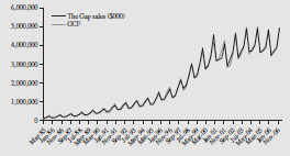
Note the very close association of the forecast with the original data as shown in the graph below: 4
Outline the different methods for combining forecast models explained in the chapter. Can more than two forecasting models be combined into a single model? Does each of the original forecasts have to be the result of the application of a quantitative technique?
Unlock Deck
Unlock for access to all 9 flashcards in this deck.
Unlock Deck
k this deck
5
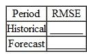
Calculate the root-mean-squared error for the historical period and comment on any improvement.
Unlock Deck
Unlock for access to all 9 flashcards in this deck.
Unlock Deck
k this deck
6
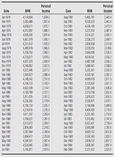
Air Carrier Traffic Statistics Monthly is a handbook of airline data published by the U.S. Department of Transportation. In this book you will find revenue passenger-miles (RPM) traveled on major airlines on international flights. Airlines regularly try to predict accurately the RPM for future periods; this gives the airline a picture of what equipment needs might be and is helpful in keeping costs at a minimum.
The revenue passenger-miles for international flights on major international airlines is shown in the accompanying table for the period Jan-1979 to Feb-1984. Also shown is personal income during the same period, in billions of dollars.
a. Build a multiple-regression model for the data to predict RPM for the next month. Check the data for any trend, and be careful to account for any seasonality. You should easily be able to obtain a forecast model with an R -squared of about 0.70 that exhibits little serial correlation.
b. Use the same data to compute a time-series decomposition model, and again forecast for one month in the future.
c. Judging from the root-mean-squared error, which of the models in parts ( a ) and ( b ) proved to be the best forecasting model? Now combine the two models, using weighting scheme like that shown in Table 8.1. Choose various weights until you believe you have come close to the optimum weighting scheme. Does this combined model perform better (according to RMSE) than either of the two original models? Why do you believe the combined model behaves in this way?
d. Try one other forecasting method of your choice on these data, and combine the results with the multiple-regression model. Do you obtain a better forecast (according to RMSE) than with either of your two original models?
The revenue passenger-miles for international flights on major international airlines is shown in the accompanying table for the period Jan-1979 to Feb-1984. Also shown is personal income during the same period, in billions of dollars.
a. Build a multiple-regression model for the data to predict RPM for the next month. Check the data for any trend, and be careful to account for any seasonality. You should easily be able to obtain a forecast model with an R -squared of about 0.70 that exhibits little serial correlation.
b. Use the same data to compute a time-series decomposition model, and again forecast for one month in the future.
c. Judging from the root-mean-squared error, which of the models in parts ( a ) and ( b ) proved to be the best forecasting model? Now combine the two models, using weighting scheme like that shown in Table 8.1. Choose various weights until you believe you have come close to the optimum weighting scheme. Does this combined model perform better (according to RMSE) than either of the two original models? Why do you believe the combined model behaves in this way?
d. Try one other forecasting method of your choice on these data, and combine the results with the multiple-regression model. Do you obtain a better forecast (according to RMSE) than with either of your two original models?
Unlock Deck
Unlock for access to all 9 flashcards in this deck.
Unlock Deck
k this deck
7
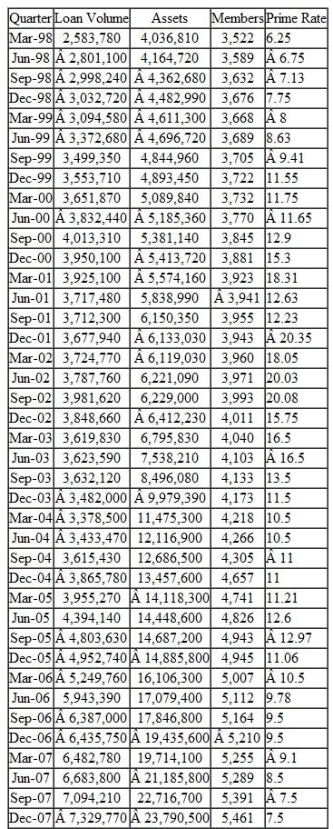
Estimating the volume of loans that will be made at a credit union is crucial to effective cash management in those institutions. In the table that follows are quarterly data for a real credit union located in a midwestern city. Credit unions are financial institutions similar to banks, but credit unions are not-for-profit firms whose members are the actual owners (remember their slogan, "It's where you belong"). The members may be both depositors in and borrowers from the credit union.
a. Estimate a multiple-regression model to estimate loan demand and calculate its root-mean- squared error.
b. Estimate a time-series decomposition model to estimate loan demand with the same data and calculate its root-mean-squared error.
c. Combine the models in parts ( a ) and ( b ) and determine whether the combined model performs better than either or both of the original models. Try to explain why you obtained the results you did.
a. Estimate a multiple-regression model to estimate loan demand and calculate its root-mean- squared error.b. Estimate a time-series decomposition model to estimate loan demand with the same data and calculate its root-mean-squared error.
c. Combine the models in parts ( a ) and ( b ) and determine whether the combined model performs better than either or both of the original models. Try to explain why you obtained the results you did.
Unlock Deck
Unlock for access to all 9 flashcards in this deck.
Unlock Deck
k this deck
8
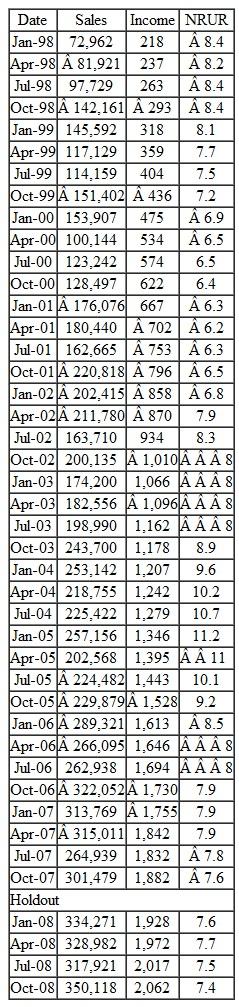
HeathCo Industries, a producer of a line of skiwear, has been the subject of exercises in several earlier chapters of the text. The data for its sales and two potential causal variables, income (INCOME) and the northern-region unemployment rate (NRUR), are repeated in the following table:
a. Develop a multiple-regression model of SALES as a function of both INCOME and NRUR:
SALES = a + b 1 (INCOME) + b 2 (NRUR)
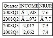
Use this model to forecast sales for 2008Q1-2008Q4 (call your regression forecast series SFR), given that INCOME and NRUR for 2004 have been forecast to be:
b. Calculate the RMSE for your regression model for both the historical period (1998Q1-2007Q4) and the forecast horizon (2008Q1-2008Q4).
d. Solely on the basis of the historical data, which model appears to be the best? Why?
e. Now prepare a combined forecast (SCF) using the regression technique described in this chapter. In the standard regression:
SALES = a + b 1 (SFR) + b 2 (SFW)
Is the intercept essentially zero? Why? If it is, do the following regression as a basis
for developing SCF:
SALES = b 1 (SFR) + b 2 (SFW)
Given the historical RMSEs found in parts ( b ) and ( c ), do the values for b 1 and b 2 seem plausible? Explain.
f. Calculate the RMSEs for SCF:
Did combining models reduce the RMSE in the historical period? What about the actual forecast?
a. Develop a multiple-regression model of SALES as a function of both INCOME and NRUR:SALES = a + b 1 (INCOME) + b 2 (NRUR)
Use this model to forecast sales for 2008Q1-2008Q4 (call your regression forecast series SFR), given that INCOME and NRUR for 2004 have been forecast to be:
b. Calculate the RMSE for your regression model for both the historical period (1998Q1-2007Q4) and the forecast horizon (2008Q1-2008Q4). d. Solely on the basis of the historical data, which model appears to be the best? Why?e. Now prepare a combined forecast (SCF) using the regression technique described in this chapter. In the standard regression:
SALES = a + b 1 (SFR) + b 2 (SFW)
Is the intercept essentially zero? Why? If it is, do the following regression as a basis
for developing SCF:
SALES = b 1 (SFR) + b 2 (SFW)
Given the historical RMSEs found in parts ( b ) and ( c ), do the values for b 1 and b 2 seem plausible? Explain.
f. Calculate the RMSEs for SCF:
Did combining models reduce the RMSE in the historical period? What about the actual forecast? Unlock Deck
Unlock for access to all 9 flashcards in this deck.
Unlock Deck
k this deck
9
Your company produces a favorite summertime food product, and you have been placed in charge of forecasting shipments of this product. The historical data below represent your company's past experience with the product.
a. Since the data appear to have both seasonality and trend, you should estimate a Winters' model and calculate its root-mean-squared error.
b. You also have access to a survey of the potential purchasers of your product. This information has been collected for some time, and it has proved to be quite accurate for predicting shipments in the past. Calculate the root-mean-squared error of the purchasers' survey data.
c. After checking for bias, combine the forecasts in parts ( a ) and ( b ) and determine if a combined model may forecast better than either single model.
a. Since the data appear to have both seasonality and trend, you should estimate a Winters' model and calculate its root-mean-squared error.
b. You also have access to a survey of the potential purchasers of your product. This information has been collected for some time, and it has proved to be quite accurate for predicting shipments in the past. Calculate the root-mean-squared error of the purchasers' survey data.
c. After checking for bias, combine the forecasts in parts ( a ) and ( b ) and determine if a combined model may forecast better than either single model.
Unlock Deck
Unlock for access to all 9 flashcards in this deck.
Unlock Deck
k this deck
Unlock Deck
Unlock for access to all 9 flashcards in this deck.


