Consider the following data:

A retail chain will buy 800 televisions if the price is $350 each and 1200 if the price is $300. A wholesaler will supply 700 of these televisions at $280 each and 1400 at $385 each.

Let us find the market equilibrium point assuming that the supply and demand functions are linear.

Convert the information in the above data into the table as follows:

Demand Quantity	Price	Supply Quantity	Price
800	350	700	280
1200	300	1400	385

First we create the demand function.

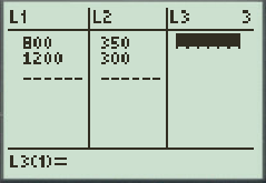
For this, enter the data of demand quantity and price from the table in the lists of a graphing utility.

The figure below shows a partial list of the data points.

The demand function, found using linear regression with a graphing calculator.

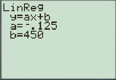
The linear equation with price p as a function of the quantity demanded q is Thus, the demand function is.