
College Algebra in Context with Applications for the Managerial, Life, and Social Sciences 3rd Edition by Ronald J Harshbarger, Lisa Yocco
النسخة 3الرقم المعياري الدولي: 032157060XCollege Algebra in Context with Applications for the Managerial, Life, and Social Sciences 3rd Edition by Ronald J Harshbarger, Lisa Yocco
النسخة 3الرقم المعياري الدولي: 032157060X تمرين 59
الحلول خطوة بخطوة موثّق
موثّق
الخطوة 1 من4
Consider that the table below gives the quantity of the graphing calculators demanded and the quantity supplied for selected prices.
| Price ($) | Quantity Demanded (thousands) | Quantity Supplied (thousands) |
| 50 | 210 | 0 |
| 60 | 190 | 40 |
| 70 | 170 | 80 |
| 80 | 150 | 120 |
| 100 | 110 | 200 |
(a) Let us find the linear equation that gives the price as a function of the quantity demanded.
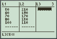
Enter the data of price and quantity demanded from the above table in the lists of a graphing utility.
The figure below shows a partial list of the data points.
The linear equation that gives the price as a function of the quantity demanded, found using linear regression with a graphing calculator.
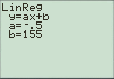
 Thus, the linear equation is
 .
. الخطوة 2 من 4
الخطوة 3 من 4
الخطوة 4 من 4
College Algebra in Context with Applications for the Managerial, Life, and Social Sciences 3rd Edition by Ronald J Harshbarger, Lisa Yocco
لماذا لم يعجبك هذا التمرين؟
أخرى 8 أحرف كحد أدنى و 255 حرفاً كحد أقصى
حرف 255


