Deck 4: Describing the Relation Between Two Variables
ملء الشاشة (f)
سؤال
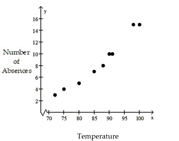
Construct a scatter diagram for the data.
-The data below are the temperatures on randomly chosen days during a summer class and the number of absences on those days.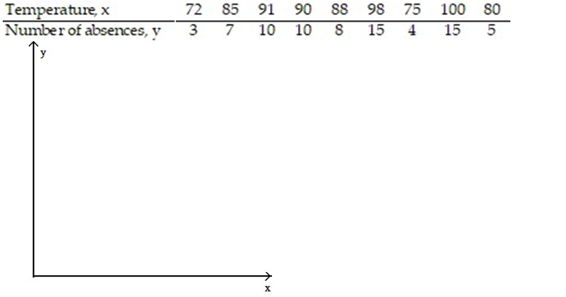
-The data below are the temperatures on randomly chosen days during a summer class and the number of absences on those days.
سؤال
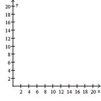
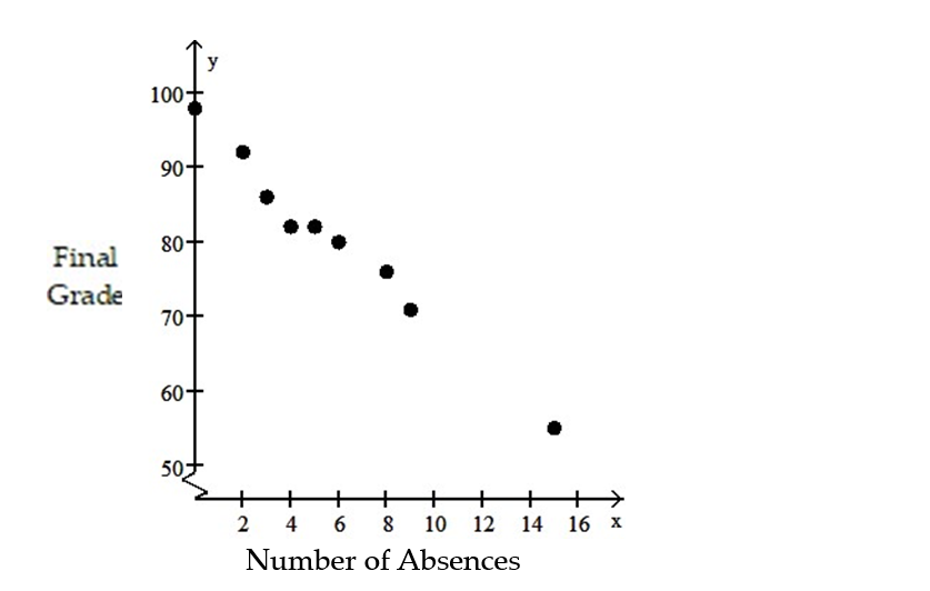
Construct a scatter diagram for the data.
-The data below are the number of absences and the final grades of 9 randomly selected students from a literature class.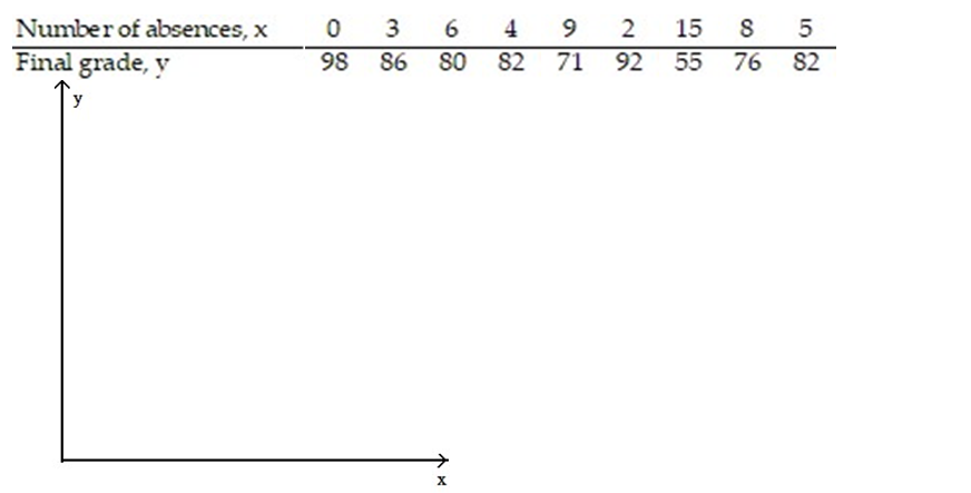
-The data below are the number of absences and the final grades of 9 randomly selected students from a literature class.
سؤال
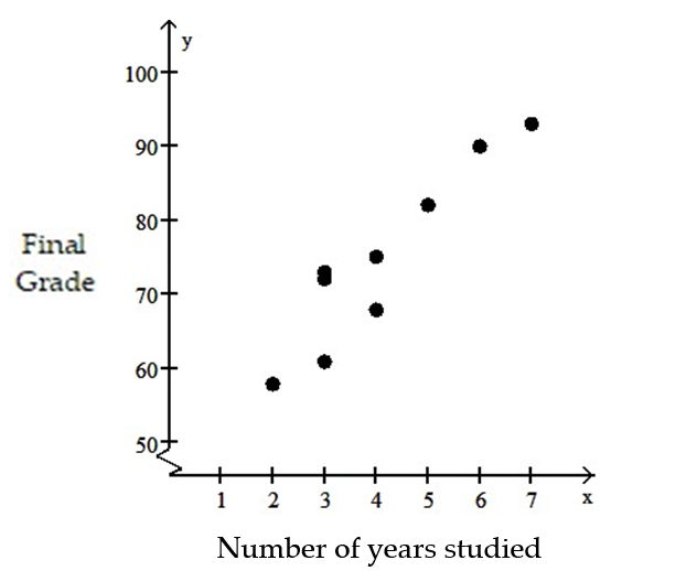
Construct a scatter diagram for the data.
-In order for employees of a company to work in a foreign office, they must take a test in the language of the country where they plan to work. The data below show the relationship between the number of years that employees have studied a particular language and the grades they received on the proficiency exam.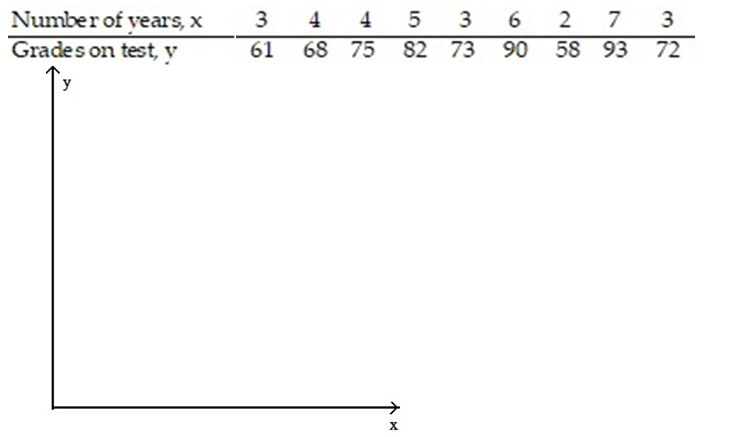
-In order for employees of a company to work in a foreign office, they must take a test in the language of the country where they plan to work. The data below show the relationship between the number of years that employees have studied a particular language and the grades they received on the proficiency exam.
سؤال
Construct a scatter diagram for the data.
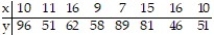
-Five brands of cigarettes were tested for the amounts of tar and nicotine they contained. All measurements are in milligrams per cigarette.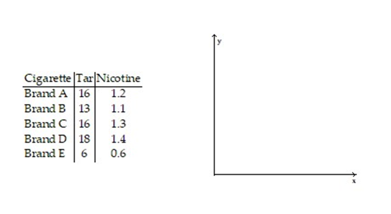
-Five brands of cigarettes were tested for the amounts of tar and nicotine they contained. All measurements are in milligrams per cigarette.
سؤال
Construct a scatter diagram for the data.
-The scores of nine members of a local community college women's golf team in two rounds of tournament play are listed below.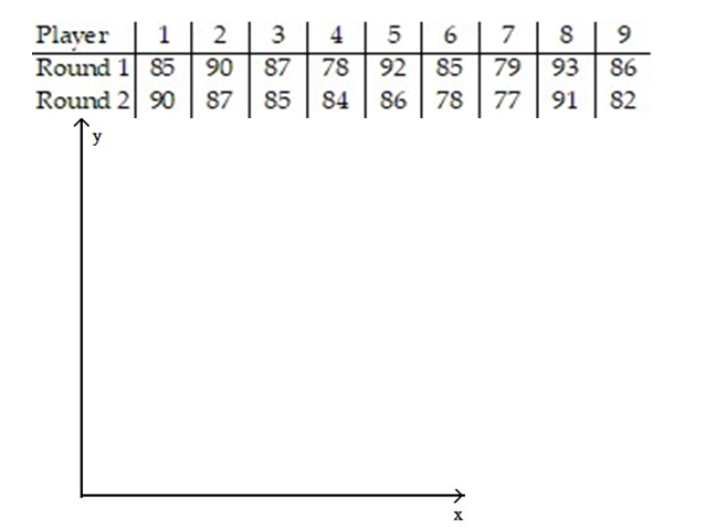
-The scores of nine members of a local community college women's golf team in two rounds of tournament play are listed below.
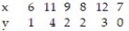
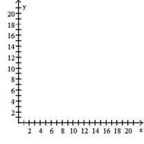
سؤال
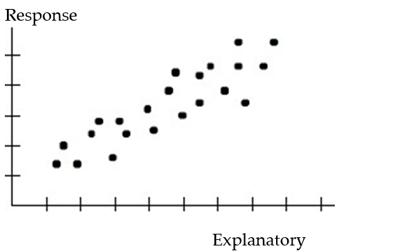
Make a scatter diagram for the data. Use the scatter diagram to describe how, if at all, the variables are related.
-
A) The variables appear to be negatively, linearly related.
B) The variables appear to be positively, linearly related.
C) The variables do not appear to be linearly related.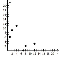
D) The variables do not appear to be linearly related.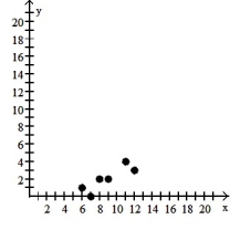
-
A) The variables appear to be negatively, linearly related.
B) The variables appear to be positively, linearly related.
C) The variables do not appear to be linearly related.
D) The variables do not appear to be linearly related.
سؤال
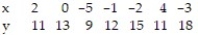
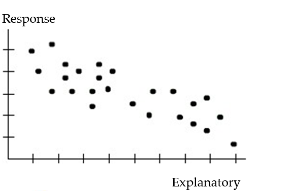
Make a scatter diagram for the data. Use the scatter diagram to describe how, if at all, the variables are related.
-
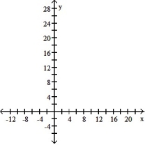
A) The variables do not appear to be linearly related.
B) The variables appear to be positively, linearly related.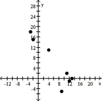
C) The variables do not appear to be linearly related.
D) The variables appear to be negatively, linearly related.
-
A) The variables do not appear to be linearly related.
B) The variables appear to be positively, linearly related.
C) The variables do not appear to be linearly related.
D) The variables appear to be negatively, linearly related.
سؤال
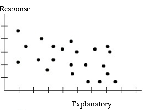
Make a scatter diagram for the data. Use the scatter diagram to describe how, if at all, the variables are related.
-
A) The variables do not appear to be linearly related.
B) The variables appear to be positively, linearly related.
C) The variables do not appear to be linearly related.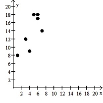
D) The variables appear to be negatively, linearly related.
-
A) The variables do not appear to be linearly related.
B) The variables appear to be positively, linearly related.
C) The variables do not appear to be linearly related.
D) The variables appear to be negatively, linearly related.
سؤال
Use the scatter diagrams shown, labeled a through f to solve the problem.
-In which scatter diagram is r = 0.01?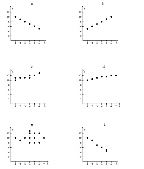
A) d
B) c
C) e
D) f
-In which scatter diagram is r = 0.01?
A) d
B) c
C) e
D) f
سؤال
The data below represent the numbers of absences and the final grades of 15 randomly selected students from an astronomy class. Construct a scatter diagram for the data. Do you detect a trend? 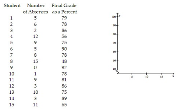
سؤال
سؤال
سؤال
سؤال
Calculate the linear correlation coefficient for the data below. 
A) 0.819
B) 0.990
C) 0.881
D) 0.792
A) 0.819
B) 0.990
C) 0.881
D) 0.792
سؤال
Calculate the linear correlation coefficient for the data below. 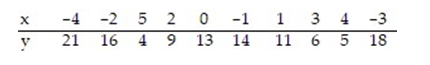
A) -0.885
B) -0.995
C) -0.671
D) -0.778
A) -0.885
B) -0.995
C) -0.671
D) -0.778
سؤال
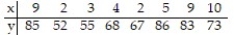
Calculate the linear correlation coefficient for the data below. 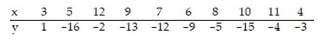
A) -0.132
B) -0.549
C) -0.104
D) -0.581
A) -0.132
B) -0.549
C) -0.104
D) -0.581
سؤال
The data below are the ages and annual pharmacy b ills (in dollars) of 9 randomly selected employees. Calculate the linear correlation coefficient. 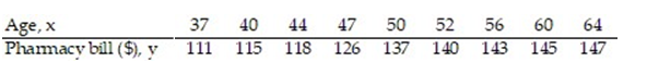
A) 0.908
B) 0.890
C) 0.960
D) 0.998
A) 0.908
B) 0.890
C) 0.960
D) 0.998
سؤال
Compute the linear correlation coefficient between the two variables and determine whether a linear relation exists.
-
A) r = 0.708; no linear relation exists
B) r = 0.235; no linear relation exists
C) r = 0.708; linear relation exists
D) r = -0.708; linear relation exists
-
A) r = 0.708; no linear relation exists
B) r = 0.235; no linear relation exists
C) r = 0.708; linear relation exists
D) r = -0.708; linear relation exists
سؤال
Compute the linear correlation coefficient between the two variables and determine whether a linear relation exists.
-
A) r = -0.335; no linear relation exists
B) r = -0.284; no linear relation exists
C) r = 0.462; linear relation exists
D) r = -0.335; linear relation exists
-
A) r = -0.335; no linear relation exists
B) r = -0.284; no linear relation exists
C) r = 0.462; linear relation exists
D) r = -0.335; linear relation exists
سؤال
Compute the linear correlation coefficient between the two variables and determine whether a linear relation exists.
-The table below shows the scores on an end-of-year project of 10 randomly selected architecture students and the number of days each student spent working on the project.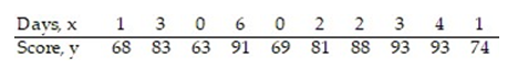
A) r = 0.847; linear relation exists
B) r = 0.761; no linear relation exists
C) r = 0.847; no linear relation exists
D) r = 0.761; linear relation exists
سؤال
Compute the linear correlation coefficient between the two variables and determine whether a linear relation exists.
-The table below shows the ages and weights (in pounds) of 9 randomly selected tennis coaches.
A) r = 0.908; linear relation exists
B) r = 0.960; no linear relation exists
C) r = 0.908; no linear relation exists
D) r = 0.960; linear relation exists
-The table below shows the ages and weights (in pounds) of 9 randomly selected tennis coaches.
A) r = 0.908; linear relation exists
B) r = 0.960; no linear relation exists
C) r = 0.908; no linear relation exists
D) r = 0.960; linear relation exists
سؤال
Compute the linear correlation coefficient between the two variables and determine whether a linear relation exists.
-To investigate the relationship between yield of soybeans and the amount of fertilizer used, a researcher divides a field into eight plots of equal size and applies a different amount of fertilizer to each plot. The table shows the yield of soybeans and the amount of fertilizer used for each plot.
A) r = 0.819; linear relation exists
B) r = 0.683; linear relation exists
C) r = 0.683; no linear relation exists
D) r = 0.729; no linear relation exists
سؤال
Find the equation of the regression line for the given data. Round values to the nearest thousandth. 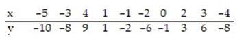
A) =0.522x-2.097
B) =-0.552x+2.097
C) =2.097x-0.552
D) =2.097x+0.552
A)
=0.522x-2.097B)
=-0.552x+2.097C)
=2.097x-0.552D)
=2.097x+0.552 سؤال
Find the equation of the regression line for the given data. Round values to the nearest thousandth. 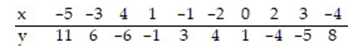
A) =-1.885x+0.758
B) =1.885x-0.758
C) =-0.758x-1.885
D) =0.758x+1.885
A)
=-1.885x+0.758B)
=1.885x-0.758C)
=-0.758x-1.885D)
=0.758x+1.885 سؤال
Find the equation of the regression line for the given data. Round values to the nearest thousandth. 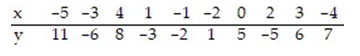
A) =2.097x-0.206
B) =-0.206x+2.097
C) =0.206x-2.097
D) =-2.097x+0.206
A)
=2.097x-0.206B)
=-0.206x+2.097C)
=0.206x-2.097D)
=-2.097x+0.206 سؤال
The data below are the average one-way commute times (in minutes) for selected students and the number of absences for those students during the term. Find the equation of the regression line for the given data. What would be the predicted number of absences if the commute time was 95 minutes? Is this a reasonable question? Round the predicted number of absences to the nearest whole number. Round the regression line values to the nearest hundredth. 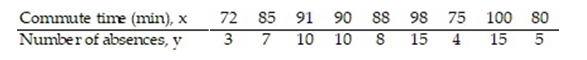
A) =0.45x-30.27; 12 absences; No, it is not reasonable. 95 minutes is well outside the scope of the model.
B) =0.45x+30.27; 73 absences; Yes, it is reasonable.
C) =0.45x+30.27; 73 absences; No, it is not reasonable. 95 minutes is well outside the scope of the model.
D) =0.45x-30.27; 12 absences; Yes, it is reasonable.
A)
=0.45x-30.27; 12 absences; No, it is not reasonable. 95 minutes is well outside the scope of the model.B)
=0.45x+30.27; 73 absences; Yes, it is reasonable.C)
=0.45x+30.27; 73 absences; No, it is not reasonable. 95 minutes is well outside the scope of the model.D)
=0.45x-30.27; 12 absences; Yes, it is reasonable. سؤال
The data below are the average one-way commute times (in minutes) for selected students and the number of absences for those students during the term. Find the equation of the regression line for the given data. What would be the predicted number of absences if the commute time was 40 minutes? Is this a reasonable question? Round the predicted number of absences to the nearest whole number. Round the regression line values to the nearest hundredth. 
A) =0.45x+30.27; 48 absences; No, it is not reasonable. 40 minutes is well outside the scope of the model.
B) =0.45x-30.27;-12 absences; No, it is not reasonable. 40 minutes is well outside the scope of the model.
C) =0.45x+30.27; 48 absences; Yes, it is reasonable.
D) =0.45x-30.27;-12 absences; Yes, it is reasonable.
A)
=0.45x+30.27; 48 absences; No, it is not reasonable. 40 minutes is well outside the scope of the model.B)
=0.45x-30.27;-12 absences; No, it is not reasonable. 40 minutes is well outside the scope of the model.C)
=0.45x+30.27; 48 absences; Yes, it is reasonable.D)
=0.45x-30.27;-12 absences; Yes, it is reasonable. سؤال
The data below are the number of absences and the final grades of 9 randomly selected students from a literature class. Find the equation of the regression line for the given data. What would be the predicted final grade if a student was absent 14 times? Round the regression line values to the nearest hundredth. Round the predicted grade to the nearest whole number. 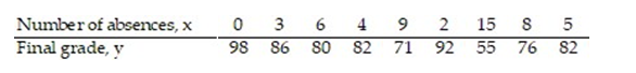
A) =96.14x-2.75; 1343
B) =-2.75x-96.14; 134.64
C) =-96.14x+2.75; 1343
D) =-2.75x+96.14; 58
A)
=96.14x-2.75; 1343B)
=-2.75x-96.14; 134.64C)
=-96.14x+2.75; 1343D)
=-2.75x+96.14; 58 سؤال
A manager wishes to determine the relationship between the number of miles traveled (in hundreds of miles) by her sales representatives and their amount of sales (in thousands of dollars) per month. Find the equation of the regression line for the given data. What would be the predicted sales if the sales representative traveled 0 miles? Is this reasonable? Why or why not? Round the regression line values to the nearest hundredth. 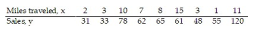
A) =3.53x+37.92; $37,920; Yes, it is reasonable.
B) =3.53x+37.92; $3792; No; it is not reasonable for a representative to travel 0 miles and have a positive amount of sales.
C) =37.92x+3.53; $3792; Yes, it is reasonable.
D) =3.53x+37.92; $37,920; No; it is not reasonable for a representative to travel 0 miles and have a positive amount of sales.
A)
=3.53x+37.92; $37,920; Yes, it is reasonable.B)
=3.53x+37.92; $3792; No; it is not reasonable for a representative to travel 0 miles and have a positive amount of sales.C)
=37.92x+3.53; $3792; Yes, it is reasonable.D)
=3.53x+37.92; $37,920; No; it is not reasonable for a representative to travel 0 miles and have a positive amount of sales. سؤال
A manager wishes to determine the relationship between the number of years her sales representatives have been employed by the firm and their amount of sales (in thousands of dollars) per month. Find the equation of the regression line for the given data. What would be the predicted sales if the sales representative was employed by the firm for 30 years Is this reasonable? Why or why not? Round the regression line values to the nearest hundredth. 
A) =3.53x+37.92; $143,820;; Yes, it is reasonable.
B) =3.53x-37.92; $67,980; No; it is not reasonable. 30 years of employment is well outside the scope of the model.
C) =3.53x-37.92; $67,980; Yes; it is reasonable.
D) =3.53x+37.92; $143,820; No; it is not reasonable. 30 years of employment is well outside the scope of the model.
A)
=3.53x+37.92; $143,820;; Yes, it is reasonable.B)
=3.53x-37.92; $67,980; No; it is not reasonable. 30 years of employment is well outside the scope of the model.C)
=3.53x-37.92; $67,980; Yes; it is reasonable.D)
=3.53x+37.92; $143,820; No; it is not reasonable. 30 years of employment is well outside the scope of the model. سؤال
The table shows, for the years 1997-2012, the mean hourly wage for residents of the town of Pity Me and the mean weekly rent paid by the residents. 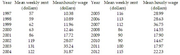 Summary statistics yield:
  = 1222.2771,
  = 3031.7125,
  = 9144.9375,
  = 21.2675, and
  Find the least squares line that uses mean hourly wage to predict mean weekly rent. Round values to the nearest ten-thousandth.
Summary statistics yield: = 1222.2771, = 3031.7125, = 9144.9375, = 21.2675, and Find the least squares line that uses mean hourly wage to predict mean weekly rent. Round values to the nearest ten-thousandth. سؤال
A county real estate appraiser wants to develop a statistical model to predict the appraised value of houses in a section of the county called East Meadow. One of the many variables thought to be an important predictor of appraised value is the number of rooms in the house. Consequently, the appraiser decided to fit the simple linear regression model,  where y = appraised value of the house (in $thousands) and x = number of rooms. Using data collected for a sample of n= 74 houses in East Meadow, the following results were obtained:
 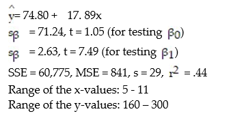 Give a practical interpretation of the estimate of the slope of the least squares line.
A) For each additional room in the house, we estimate the appraised value to increase $ 17, 890.
B) For each additional dollar of appraised value, we estimate the number of rooms in the house to increase by 17. 89 rooms.
C) For each additional room in the house, we estimate the appraised value to increase $74,800.
D) For a house with 0 rooms, we estimate the appraised value to be $74,800.
where y = appraised value of the house (in $thousands) and x = number of rooms. Using data collected for a sample of n= 74 houses in East Meadow, the following results were obtained: Give a practical interpretation of the estimate of the slope of the least squares line.A) For each additional room in the house, we estimate the appraised value to increase $ 17, 890.
B) For each additional dollar of appraised value, we estimate the number of rooms in the house to increase by 17. 89 rooms.
C) For each additional room in the house, we estimate the appraised value to increase $74,800.
D) For a house with 0 rooms, we estimate the appraised value to be $74,800.
سؤال
A county real estate appraiser wants to develop a statistical model to predict the appraised value of houses in a section of the county called East Meadow. One of the many variables thought to be an important predictor of appraised value is the number of rooms in the house. Consequently, the appraiser decided to fit the simple linear regression model,  where y = appraised value of the house (in $thousands) and x = number of rooms. Using data collected for a sample of n= 74 houses in East Meadow, the following results were obtained:
 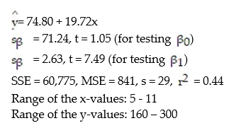 Give a practical interpretation of the estimate of the y-intercept of the least squares line.
A) For each additional room in the house, we estimate the appraised value to increase $19,720.
B) For each additional room in the house, we estimate the appraised value to increase $74,800.
C) There is no practical interpretation, since a house with 0 rooms is nonsensical.
D) We estimate the base appraised value for any house to be $74,800.
where y = appraised value of the house (in $thousands) and x = number of rooms. Using data collected for a sample of n= 74 houses in East Meadow, the following results were obtained: Give a practical interpretation of the estimate of the y-intercept of the least squares line.A) For each additional room in the house, we estimate the appraised value to increase $19,720.
B) For each additional room in the house, we estimate the appraised value to increase $74,800.
C) There is no practical interpretation, since a house with 0 rooms is nonsensical.
D) We estimate the base appraised value for any house to be $74,800.
سؤال
Is there a relationship between the raises administrators at State University receive and their performance on the job? A faculty group wants to determine whether job rating (x) is a useful linear predictor of raise (y). Consequently, the group considered the straight-line regression model,  Using the method of least squares, the faculty group obtained the following prediction equation,
  Interpret the estimated slope of the line.
A) For a $1 increase in an administrator's raise, we estimate the administrator's rating to decrease 2,000 points.
B) For a 1-point increase in an administrator's rating, we estimate the administrator's raise to decrease $2,000.
C) For a 1-point increase in an administrator's rating, we estimate the administrator's raise to increase $2,000.
D) For an administrator with a rating of 1.0, we estimate his/her raise to be $2,000.
Using the method of least squares, the faculty group obtained the following prediction equation, Interpret the estimated slope of the line.A) For a $1 increase in an administrator's raise, we estimate the administrator's rating to decrease 2,000 points.
B) For a 1-point increase in an administrator's rating, we estimate the administrator's raise to decrease $2,000.
C) For a 1-point increase in an administrator's rating, we estimate the administrator's raise to increase $2,000.
D) For an administrator with a rating of 1.0, we estimate his/her raise to be $2,000.
سؤال
Is there a relationship between the raises administrators at State University receive and their performance on the job? A faculty group wants to determine whether job rating (x) is a useful linear predictor of raise (y). Consequently, the group considered the straight-line regression model,  Using the method of least squares, the faculty group obtained the following prediction equation,
 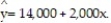 Interpret the estimated y-intercept of the line.
A) The base administrator raise at State University is $14,000.
B) For a 1-point increase in an administrator's rating, we estimate the administrator's raise to increase $14,000.
C) There is no practical interpretation, since rating of 0 is nonsensical and outside the range of the sample data.
D) For an administrator who receives a rating of zero, we estimate his or her raise to be $14,000.
Using the method of least squares, the faculty group obtained the following prediction equation, Interpret the estimated y-intercept of the line.A) The base administrator raise at State University is $14,000.
B) For a 1-point increase in an administrator's rating, we estimate the administrator's raise to increase $14,000.
C) There is no practical interpretation, since rating of 0 is nonsensical and outside the range of the sample data.
D) For an administrator who receives a rating of zero, we estimate his or her raise to be $14,000.
سؤال
A large national bank charges local companies for using its services. A bank official reported the results of a regression analysis designed to predict the bank's charges (y), measured in dollars per month, for services rendered to local companies. One independent variable used to predict service charge to a company is the company's sales revenue (x), measured in millions of dollars. Data for 21 companies who use the bank's services were used to fit the model,  The results of the simple linear regression are provided below.
  = 2,700 + 20x, s = 65, 2-tailed p-value = 0.064 (for testing
  )Interpret the estimate of
  , the y-intercept of the line.
A) All companies will be charged at least $2,700 by the bank.
B) About 95% of the observed service charges fall within $2,700 of the least squares line.
C) There is no practical interpretation since a sales revenue of $0 is a nonsensical value.
D) For every $1 million increase in sales revenue, we expect a service charge to increase $2,700.
The results of the simple linear regression are provided below. = 2,700 + 20x, s = 65, 2-tailed p-value = 0.064 (for testing )Interpret the estimate of , the y-intercept of the line.A) All companies will be charged at least $2,700 by the bank.
B) About 95% of the observed service charges fall within $2,700 of the least squares line.
C) There is no practical interpretation since a sales revenue of $0 is a nonsensical value.
D) For every $1 million increase in sales revenue, we expect a service charge to increase $2,700.
سؤال
Civil engineers often use the straight-line equation,  =
=  +
+  x, to model the relationship between the mean shear strength of masonry joints and precompression stress, x. To test this theory, a series of stress tests were performed on solid bricks arranged in triplets and joined with mortar. The precompression stress was varied for each triplet and the ultimate shear load just before failure (called the shear strength) was recorded. The stress results for n = 7 triplet tests is shown in the accompanying table followed by a SAS printout of the regression analysis.
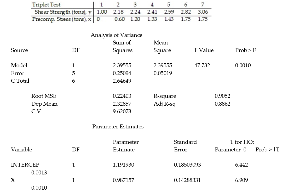
-Give a practical interpretation of the estimate of the slope of the least squares line.
A) For a triplet test with a precompression stress of 1 ton, we estimate the shear strength of the joint to be 0.987 ton.
B) For every 0.987 ton increase in precompression stress, we estimate the shear strength of the joint to increase by 1 ton.
C) For a triplet test with a precompression stress of 0 tons, we estimate the shear strength of the joint to be 1.19 tons.
D) For every 1 ton increase in precompression stress, we estimate the shear strength of the joint to increase by 0.987 ton.
= + x, to model the relationship between the mean shear strength of masonry joints and precompression stress, x. To test this theory, a series of stress tests were performed on solid bricks arranged in triplets and joined with mortar. The precompression stress was varied for each triplet and the ultimate shear load just before failure (called the shear strength) was recorded. The stress results for n = 7 triplet tests is shown in the accompanying table followed by a SAS printout of the regression analysis. -Give a practical interpretation of the estimate of the slope of the least squares line.
A) For a triplet test with a precompression stress of 1 ton, we estimate the shear strength of the joint to be 0.987 ton.
B) For every 0.987 ton increase in precompression stress, we estimate the shear strength of the joint to increase by 1 ton.
C) For a triplet test with a precompression stress of 0 tons, we estimate the shear strength of the joint to be 1.19 tons.
D) For every 1 ton increase in precompression stress, we estimate the shear strength of the joint to increase by 0.987 ton.
سؤال
Civil engineers often use the straight-line equation,  =
=  +
+  x, to model the relationship between the mean shear strength of masonry joints and precompression stress, x. To test this theory, a series of stress tests were performed on solid bricks arranged in triplets and joined with mortar. The precompression stress was varied for each triplet and the ultimate shear load just before failure (called the shear strength) was recorded. The stress results for n = 7 triplet tests is shown in the accompanying table followed by a SAS printout of the regression analysis.
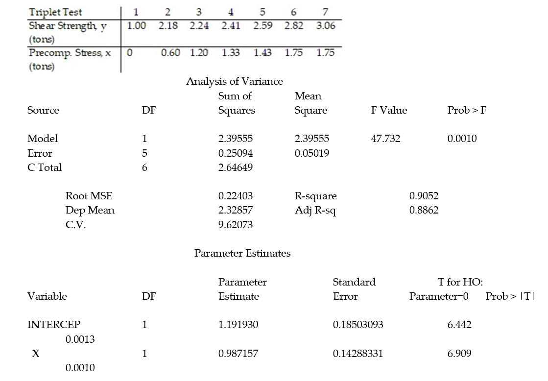
- Give a practical interpretation of the estimate of the y-intercept of the least squares line.
A) For a triplet test with a precompression stress of 0 tons, we estimate the shear strength of the joint to increase 1.19 tons.
B) There is no practical interpretation since a triplet test with a precompression stress of 0 tons is outside the range of the sample data.
C) For a triplet test with a precompression stress of 0 tons, we estimate the shear strength of the joint to be 1.19 tons.
D) For every 1 ton increase in precompression stress, we estimate the shear strength of the joint to increase by 0.987 ton.
= + x, to model the relationship between the mean shear strength of masonry joints and precompression stress, x. To test this theory, a series of stress tests were performed on solid bricks arranged in triplets and joined with mortar. The precompression stress was varied for each triplet and the ultimate shear load just before failure (called the shear strength) was recorded. The stress results for n = 7 triplet tests is shown in the accompanying table followed by a SAS printout of the regression analysis. - Give a practical interpretation of the estimate of the y-intercept of the least squares line.
A) For a triplet test with a precompression stress of 0 tons, we estimate the shear strength of the joint to increase 1.19 tons.
B) There is no practical interpretation since a triplet test with a precompression stress of 0 tons is outside the range of the sample data.
C) For a triplet test with a precompression stress of 0 tons, we estimate the shear strength of the joint to be 1.19 tons.
D) For every 1 ton increase in precompression stress, we estimate the shear strength of the joint to increase by 0.987 ton.
سؤال
Each year a nationally recognized publication conducts its "Survey of America's Best Graduate and Professional Schools." An academic advisor wants to predict the typical starting salary of a graduate at a top business school using GMAT score of the school as a predictor variable. Total GMAT scores range from 200 to 800. A simple linear regression of SALARY versus GMAT using 25 data points shown below. 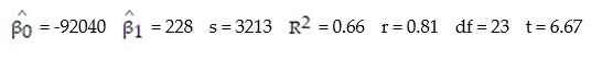
-Give a practical interpretation of = -92040.
A) We expect to predict SALARY to within 2(92040) = $184,080 of its true value using GMAT in a straight-line model.
B) We estimate the base SALARY of graduates of a top business school to be $-92,040.
C) We estimate SALARY to decrease $92,040 for every 1-point increase in GMAT.
D) The value has no practical interpretation since a GMAT of 0 is nonsensical and outside the range of the sample data.
-Give a practical interpretation of
= -92040.A) We expect to predict SALARY to within 2(92040) = $184,080 of its true value using GMAT in a straight-line model.
B) We estimate the base SALARY of graduates of a top business school to be $-92,040.
C) We estimate SALARY to decrease $92,040 for every 1-point increase in GMAT.
D) The value has no practical interpretation since a GMAT of 0 is nonsensical and outside the range of the sample data.
سؤال
Each year a nationally recognized publication conducts its "Survey of America's Best Graduate and Professional Schools." An academic advisor wants to predict the typical starting salary of a graduate at a top business school using GMAT score of the school as a predictor variable. Total GMAT scores range from 200 to 800. A simple linear regression of SALARY versus GMAT using 25 data points shown below. 
-Give a practical interpretation of = 228.
A) We expect to predict SALARY to within 2(228) = $456 of its true value using GMAT in a straight-line model.
B) The value has no practical interpretation since a GMAT of 0 is nonsensical and outside the range of the sample data.
C) We estimate SALARY to increase $228 for every 1-point increase in GMAT.
D) We estimate GMAT to increase 228 points for every $1 increase in SALARY.
-Give a practical interpretation of
= 228.A) We expect to predict SALARY to within 2(228) = $456 of its true value using GMAT in a straight-line model.
B) The value has no practical interpretation since a GMAT of 0 is nonsensical and outside the range of the sample data.
C) We estimate SALARY to increase $228 for every 1-point increase in GMAT.
D) We estimate GMAT to increase 228 points for every $1 increase in SALARY.
سؤال
A real estate magazine reported the results of a regression analysis designed to predict the price (y), measured in dollars, of residential properties recently sold in a northern Virginia subdivision. One independent variable used to predict sale price is GLA, gross living area (x), measured in square feet. Data for 157 properties were used to fit the model,  =
=  +
+  x. The results of the simple linear regression are provided below.
 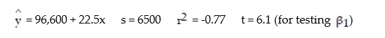 Interpret the estimate of
  , the y-intercept of the line.
A) For every 1-sq ft. increase in GLA, we expect a property's sale price to increase $96,600.
B) About 95% of the observed sale prices fall within $96,600 of the least squares line.
C) There is no practical interpretation, since a gross living area of 0 is a nonsensical value.
D) All residential properties in Virginia will sell for at least $96,600.
= + x. The results of the simple linear regression are provided below. Interpret the estimate of , the y-intercept of the line.A) For every 1-sq ft. increase in GLA, we expect a property's sale price to increase $96,600.
B) About 95% of the observed sale prices fall within $96,600 of the least squares line.
C) There is no practical interpretation, since a gross living area of 0 is a nonsensical value.
D) All residential properties in Virginia will sell for at least $96,600.
سؤال
In a comprehensive road test on all new car models, one variable measured is the time it takes a car to accelerate from 0 to 60 miles per hour. To model acceleration time, a regression analysis is conducted on a random sample of 129 new cars.
TIME60: y = Elapsed time (in seconds) from 0 mph to 60 mph
MAX: = Maximum speed attained (miles per hour)
Initially, the simple linear model E(y) = +
+ 
 was fit to the data. Computer printouts for the analysis are given below:
 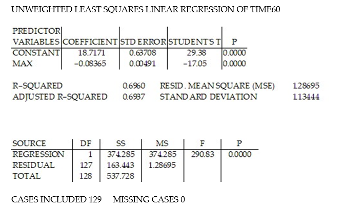 Find and interpret the estimate
  in the printout above.
TIME60: y = Elapsed time (in seconds) from 0 mph to 60 mph
MAX:
= Maximum speed attained (miles per hour)Initially, the simple linear model E(y) =
+ was fit to the data. Computer printouts for the analysis are given below: Find and interpret the estimate in the printout above. سؤال
In a study of feeding behavior, zoologists recorded the number of grunts of a warthog feeding by a lake in the 15 minute period following the addition of food. The data showing the weekly number of grunts and the age of the warthog (in days) are listed below: 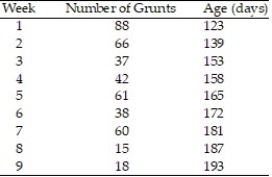 a. Write the equation of a straight-line model relating number of grunts (y) to age (x).
b. Give the least squares prediction equation.
c. Give a practical interpretation of the value of if possible.
d. Give a practical interpretation of the value of if possible.
a. Write the equation of a straight-line model relating number of grunts (y) to age (x).b. Give the least squares prediction equation.
c. Give a practical interpretation of the value of
if possible.d. Give a practical interpretation of the value of
if possible. سؤال
Given the equation of a regression line is  = -5.5x - 0.7, what is the best predicted value for y given x= 7.4?
A) 40.00
B) 41.40
C) -41.40
D) -40.00
= -5.5x - 0.7, what is the best predicted value for y given x= 7.4?A) 40.00
B) 41.40
C) -41.40
D) -40.00
سؤال
Use the regression equation to predict the value of y for x = -3.4. 
A) -7.682
B) 3.974
C) 0.220
D) -6.578
A) -7.682
B) 3.974
C) 0.220
D) -6.578
سؤال
Use the regression equation to predict the value of y for x = -1.1. 
A) 1.051
B) -2.719
C) -1.315
D) 2.832
A) 1.051
B) -2.719
C) -1.315
D) 2.832
سؤال
In an area of the Great Plains, records were kept on the relationship between the rainfall (in inches) and the yield of wheat (bushels per acre). Which is the best predicted value for y given x = 18.1? 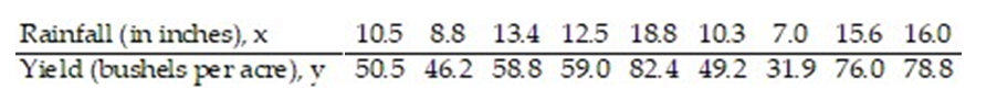
A) 83.3
B) 83.5
C) 84.0
D) 83.8
A) 83.3
B) 83.5
C) 84.0
D) 83.8
سؤال
A calculus instructor is interested in finding the strength of a relationship between the final exam grades of students enrolled in Calculus I and Calculus II at his college. The data (in percentages) are listed below. 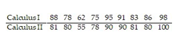 a) Graph a scatter diagram of the data.
b) Find an equation of the regression line.
c) Predict a Calculus II exam score for a student who receives an 80 in Calculus I.
a) Graph a scatter diagram of the data.b) Find an equation of the regression line.
c) Predict a Calculus II exam score for a student who receives an 80 in Calculus I.
سؤال
In one area of Russia, records were kept on the relationship between the rainfall (in inches) and the yield of wheat (bushels per acre). The data for a 9 year period is as follows: 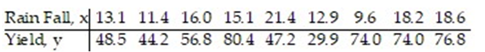 The equation of the line of least squares is given as
  = -9.12 + 4.38x.
-How many bushels of wheat per acre can be predicted if it is expected that there will be 17 inches of rain?
A) 5.96
B) 61.18
C) 65.34
D) 52.06
The equation of the line of least squares is given as = -9.12 + 4.38x. -How many bushels of wheat per acre can be predicted if it is expected that there will be 17 inches of rain?
A) 5.96
B) 61.18
C) 65.34
D) 52.06
سؤال
In an area of Russia, records were kept on the relationship between the rainfall (in inches) and the yield of wheat (bushels per acre). The data for a 9 year period is as follows:  The equation of the line of least squares is given as
  = -9.12 + 4.38x.
-What would be the expected number of inches of rain if the yield is 60 bushels of wheat per acre?
A) 64.74
B) 253.68
C) 11.62
D) 15.78
The equation of the line of least squares is given as = -9.12 + 4.38x. -What would be the expected number of inches of rain if the yield is 60 bushels of wheat per acre?
A) 64.74
B) 253.68
C) 11.62
D) 15.78
سؤال
In an area of Russia, records were kept on the relationship between the rainfall (in inches) and the yield of wheat (bushels per acre). The data for a 9 year period is as follows:  The equation of the line of least squares is given as
  = -9.12 + 4.38x.
- How many bushels of wheat per acre can be predicted if it is expected that there will be 30 inches of rain?
A) Cannot be certain of the result because 30 inches of rain exceeds the observed data.
B) 8.93
C) 122.28
D) 140.52
The equation of the line of least squares is given as = -9.12 + 4.38x.- How many bushels of wheat per acre can be predicted if it is expected that there will be 30 inches of rain?
A) Cannot be certain of the result because 30 inches of rain exceeds the observed data.
B) 8.93
C) 122.28
D) 140.52
سؤال
The regression line for the given data is  = 2.097x - 0.552. Determine the residual of a data point for which x = 3 and y = 6.
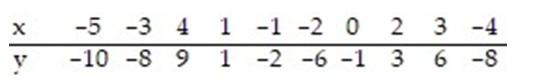
A) 5.739
B) -9.03
C) 11.739
D) 0.261
= 2.097x - 0.552. Determine the residual of a data point for which x = 3 and y = 6. A) 5.739
B) -9.03
C) 11.739
D) 0.261
سؤال
The regression line for the given data is  = -1.885x + 0.758. Determine the residual of a data point for which x = 4 and y = -6.
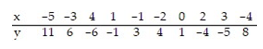
A) -12.782
B) -8.068
C) 0.782
D) -6.782
= -1.885x + 0.758. Determine the residual of a data point for which x = 4 and y = -6. A) -12.782
B) -8.068
C) 0.782
D) -6.782
سؤال
The regression line for the given data is  = -0.206x + 2.097. Determine the residual of a data point for which x = 0 and y = 5.
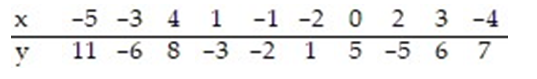
A) 2.097
B) 7.097
C) 2.903
D) -1.067
= -0.206x + 2.097. Determine the residual of a data point for which x = 0 and y = 5. A) 2.097
B) 7.097
C) 2.903
D) -1.067
سؤال
The regression line for the given data is  = 5.044x + 56.11. Determine the residual of a data point for which x = 4 and y = 78.
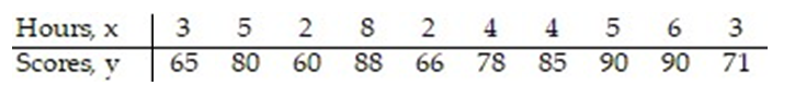
A) 154.286
B) 76.286
C) -445.542
D) 1.714
= 5.044x + 56.11. Determine the residual of a data point for which x = 4 and y = 78. A) 154.286
B) 76.286
C) -445.542
D) 1.714
سؤال
The regression line for the given data is  = 0.449x - 30.27. Determine the residual of a data point for which x = 100 and y = 15.
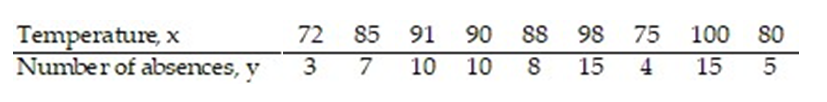
A) 14.63
B) 0.37
C) 29.63
D) 123.535
= 0.449x - 30.27. Determine the residual of a data point for which x = 100 and y = 15. A) 14.63
B) 0.37
C) 29.63
D) 123.535
سؤال
The regression line for the given data is  = 1.488x + 60.46. Determine the residual of a data point for which x = 41 and y = 120.
A) -1.468
B) -198.02
C) 241.468
D) 121.468
= 1.488x + 60.46. Determine the residual of a data point for which x = 41 and y = 120. A) -1.468
B) -198.02
C) 241.468
D) 121.468
سؤال
The regression line for the given data is  = -2.75x + 96.14. Determine the residual of a data point for which x = 0 and y = 98.
A) 173.36
B) 96.14
C) 194.14
D) 1.86
= -2.75x + 96.14. Determine the residual of a data point for which x = 0 and y = 98. A) 173.36
B) 96.14
C) 194.14
D) 1.86
سؤال
The regression line for the given data is  = 3.53x + 37.92. Determine the residual of a data point for which x = 8 and y = 65.
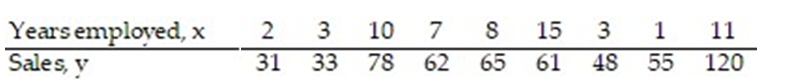
A) 66.16
B) 131.16
C) -259.37
D) -1.16
= 3.53x + 37.92. Determine the residual of a data point for which x = 8 and y = 65. A) 66.16
B) 131.16
C) -259.37
D) -1.16
سؤال
The regression line for the given data is  = 6.91x + 46.26. Determine the residual of a data point for which x = 2 and y = 58.
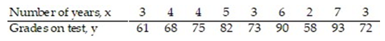
A) 118.08
B) -2.08
C) 60.08
D) -445.04
= 6.91x + 46.26. Determine the residual of a data point for which x = 2 and y = 58. A) 118.08
B) -2.08
C) 60.08
D) -445.04
سؤال
The regression line for the given data is  = 4.379x + 4.267. Determine the residual of a data point for which x = 10.5 and y = 50.5.
A) 50.2465
B) 100.7465
C) 0.2535
D) -214.9065
= 4.379x + 4.267. Determine the residual of a data point for which x = 10.5 and y = 50.5. A) 50.2465
B) 100.7465
C) 0.2535
D) -214.9065
سؤال
Compute the sum of the squared residuals of the least-squares line for the given data. 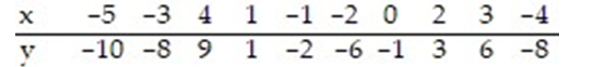
A) 0
B) 2.097
C) 7.624
D) 1.036
A) 0
B) 2.097
C) 7.624
D) 1.036
سؤال
In a study of feeding behavior, zoologists recorded the number of grunts of a warthog feeding by a lake in a 15 minute time period following the addition of food. The data showing the weekly number of grunts and the age of the warthog (in days) are listed below. Compute the sum of the squared residuals of the least squared line for the given data. 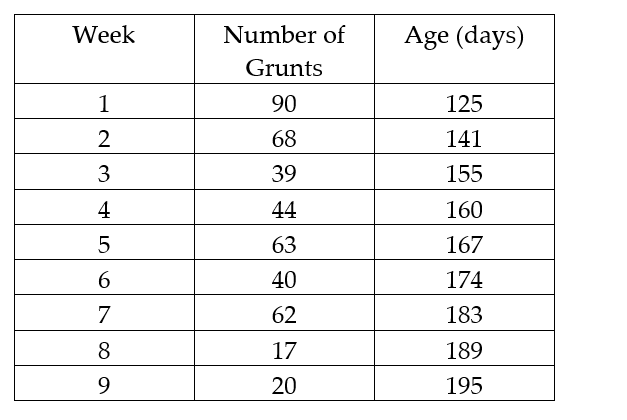
A) 13.74
B) 188.84
C) 74.39
D) 5533.53
A) 13.74
B) 188.84
C) 74.39
D) 5533.53
سؤال
The data below are the ages and systolic blood pressure (measured in Millimeters of mercury) of 9 randomly selected adults. 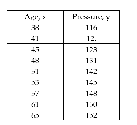
A) 123.63
B) 1.41
C) 11.11
D) 1.99
A) 123.63
B) 1.41
C) 11.11
D) 1.99
سؤال
Choose the coefficient of determination that matches the scatterplot. Assume that the scales on the horizontal and vertical axes are the same.
-
A) =0.96
=0.96
B) =0.77
=0.77
C) =0.38
=0.38
D) =0.51
=0.51
-
A)
=0.96B)
=0.77C)
=0.38D)
=0.51 سؤال
Choose the coefficient of determination that matches the scatterplot. Assume that the scales on the horizontal and vertical axes are the same.
-
A) =0.12
=0.12
B) =0.82
=0.82
C) =0.43
=0.43
D) =-0.43
-
A)
=0.12B)
=0.82C)
=0.43D)
=-0.43 سؤال
Choose the coefficient of determination that matches the scatterplot. Assume that the scales on the horizontal and vertical axes are the same.
-
A) =0.76
=0.76
B) =0.41
=0.41
C) =-0.31
D) =0.097
-
A)
=0.76B)
=0.41C)
=-0.31D)
=0.097 سؤال
Use the linear correlation coefficient given to determine the coefficient of determination , 
-r = 0.32
A) =56.57%
B) =5.66%
C) =10.24%
D) =1.024%
-r = 0.32
A)
=56.57%B)
=5.66%C)
=10.24%D)
=1.024% سؤال
Use the linear correlation coefficient given to determine the coefficient of determination ,
-r = -0.42
A) =-17.64%
B) =17.64%
C) =-64.81%
D) =64.81%
-r = -0.42
A)
=-17.64%B)
=17.64%C)
=-64.81%D)
=64.81% سؤال
In a study of feeding behavior, zoologists recorded the number of grunts of a warthog feeding by a lake in the 15 minute period following the addition of food. The data showing the weekly number of grunts and the age of the warthog (in days) are listed below. Find and interpret the value of  . Round
  to the nearest thousandth.
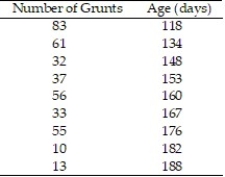
. Round to the nearest thousandth. سؤال
In a comprehensive road test on all new car models, one variable measured is the time it takes a car to accelerate from 0 to 60 miles per hour. To model acceleration time, a regression analysis is conducted on a random sample of 129 new cars. 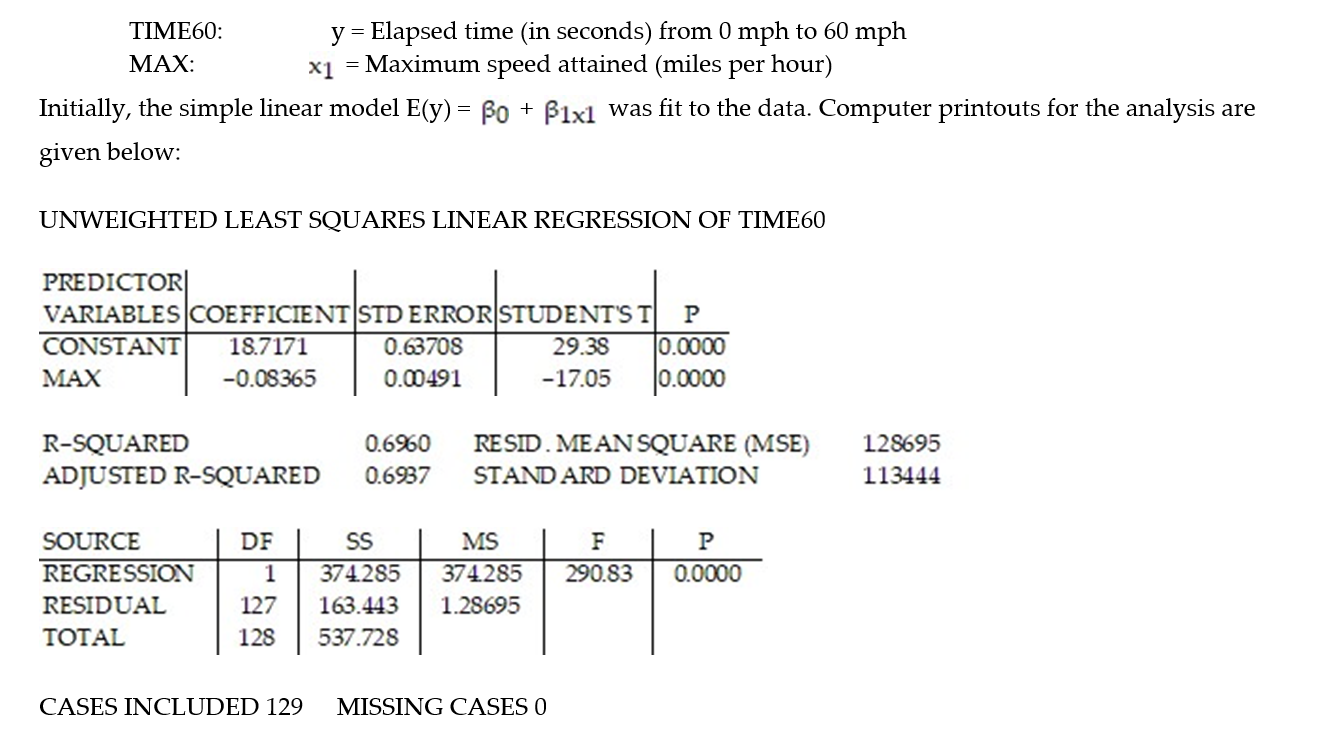 Approximately what percentage, rounded to the nearest whole percent, of the sample variation in acceleration time can be explained by the simple linear model?
A) 8%
B) 70%
C) -17%
D) 0%
Approximately what percentage, rounded to the nearest whole percent, of the sample variation in acceleration time can be explained by the simple linear model?A) 8%
B) 70%
C) -17%
D) 0%
سؤال
A manufacturer of boiler drums wants to use regression to predict the number of man-hours needed to erect drums in the future. The manufacturer collected a random sample of 35 boilers and measured the following two variables: 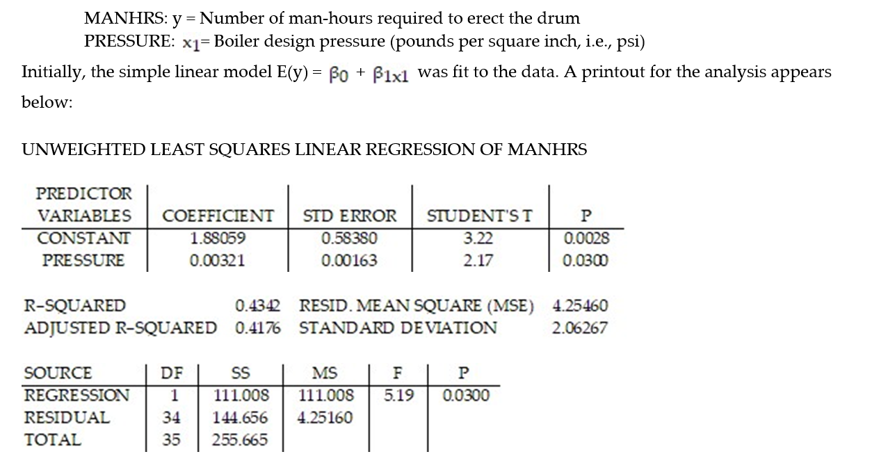 Give a practical interpretation of the coefficient of determination,
  . Express
  to the nearest whole percent.
A) About 43% of the sample variation in number of man-hours can be explained by the simple linear model.
B) About 2.06% of the sample variation in number of man-hours can be explained by the simple linear model.
C) Man hours needed to erect drums will be associated with boiler design pressure 43% of the time.
D) =1.88+0.00321x will be correct 43% of the time.
Give a practical interpretation of the coefficient of determination, . Express to the nearest whole percent.A) About 43% of the sample variation in number of man-hours can be explained by the simple linear model.
B) About 2.06% of the sample variation in number of man-hours can be explained by the simple linear model.
C) Man hours needed to erect drums will be associated with boiler design pressure 43% of the time.
D)
=1.88+0.00321x will be correct 43% of the time. سؤال
Civil engineers often use the straight-line equation, E(y) =  +
+  x, to model the relationship between the mean shear strength E(y) of masonry joints and precompression stress, x. To test this theory, a series of stress tests were performed on solid bricks arranged in triplets and joined with mortar. The precompression stress was varied for each triplet and the ultimate shear load just before failure (called the shear strength) was recorded. The stress results for n = 7 triplet tests is shown in the accompanying table followed by a SAS printout of the regression analysis.
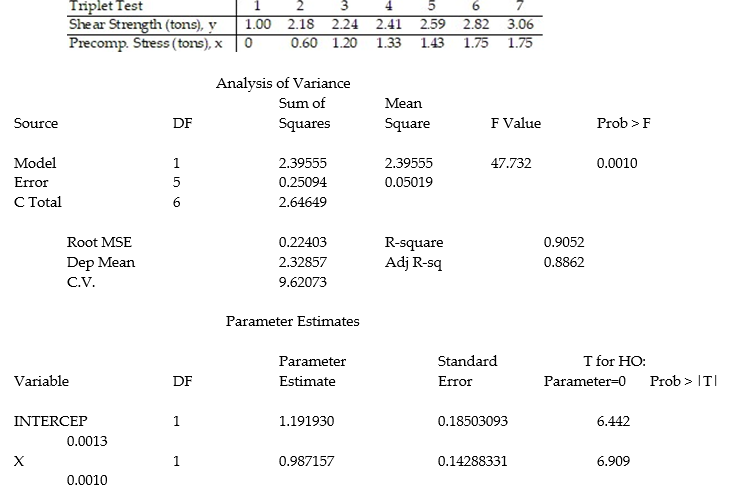
A) In repeated sampling, approximately 91% of all similarly constructed regression lines will accurately predict shear strength.
B) About 91% of the total variation in the sample of y-values can be explained by (or attributed to) the linear relationship between shear strength and precompression stress.
C) We expect about 91% of the observed shear strength values to lie on the least squares line.
D) We expect to predict the shear strength of a triplet test to within about .91 ton of its true value.
+ x, to model the relationship between the mean shear strength E(y) of masonry joints and precompression stress, x. To test this theory, a series of stress tests were performed on solid bricks arranged in triplets and joined with mortar. The precompression stress was varied for each triplet and the ultimate shear load just before failure (called the shear strength) was recorded. The stress results for n = 7 triplet tests is shown in the accompanying table followed by a SAS printout of the regression analysis. A) In repeated sampling, approximately 91% of all similarly constructed regression lines will accurately predict shear strength.
B) About 91% of the total variation in the sample of y-values can be explained by (or attributed to) the linear relationship between shear strength and precompression stress.
C) We expect about 91% of the observed shear strength values to lie on the least squares line.
D) We expect to predict the shear strength of a triplet test to within about .91 ton of its true value.
سؤال
The dean of the Business School at a small Florida college wishes to determine whether the grade-point average (GPA) of a graduating student can be used to predict the graduate's starting salary. More specifically, the dean wants to know whether higher GPA's lead to higher starting salaries. Records for 23 of last year's Business School graduates are selected at random, and data on GPA (x) and starting salary (y, in $thousands) for each graduate were used to fit the model, E(y) =  +
+  x. The results of the simple linear regression are provided below.
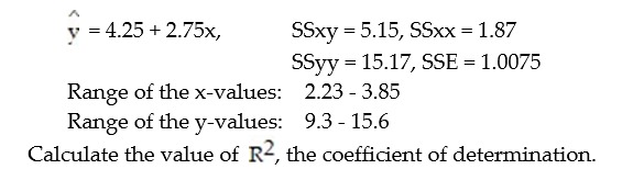
A) 0.934
B) 0.872
C) 0.339
D) 0.661
+ x. The results of the simple linear regression are provided below. A) 0.934
B) 0.872
C) 0.339
D) 0.661
سؤال
Each year a nationally recognized publication conducts its "Survey of America's Best Graduate and Professional Schools." An academic advisor wants to predict the typical starting salary of a graduate at a top business school using GMAT score of the school as a predictor variable. A simple linear regression of SALARY versus GMAT using 25 data points shown below. 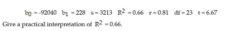
A) We can predict SALARY correctly 66% of the time using GMAT in a straight-line model.
B) 66% of the differences in SALARY are caused by differences in GMAT scores.
C) 66% of the sample variation in SALARY can be explained by using GMAT in a straight-line model.
D) We estimate SALARY to increase $.66 for every 1-point increase in GMAT.
سؤال
A real estate magazine reported the results of a regression analysis designed to predict the price (y), measured in dollars, of residential properties recently sold in a northern Virginia subdivision. One independent variable used to predict sale price is GLA, gross living area (x), measured in square feet. Data for 157 properties were used to fit the model, E(y) =  +
+  x. The results of the simple linear regression are provided below.
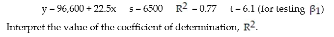
A) 77% of the total variation in the sample sale prices can be attributed to the linear relationship between GLA (x) and (y).
B) There is a moderately strong positive correlation between sale price (y) and GLA (x).
C) 77% of the observed sale prices (y's) will fall within 2 standard deviations of the least squares line.
D) GLA (x) is linearly related to sale price (y) 77% of the time.
+ x. The results of the simple linear regression are provided below. A) 77% of the total variation in the sample sale prices can be attributed to the linear relationship between GLA (x) and (y).
B) There is a moderately strong positive correlation between sale price (y) and GLA (x).
C) 77% of the observed sale prices (y's) will fall within 2 standard deviations of the least squares line.
D) GLA (x) is linearly related to sale price (y) 77% of the time.
سؤال
A company keeps extensive records on its new salespeople on the premise that sales should increase with experience. A random sample of seven new salespeople produced the data on experience and sales shown in the table. 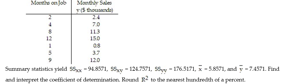
سؤال
To investigate the relationship between yield of potatoes, y, and level of fertilizer application, x, an experimenter divides a field into eight plots of equal size and applies differing amounts of fertilizer to each. The yield of potatoes (in pounds) and the fertilizer application (in pounds) are recorded for each plot. The data are as follows: 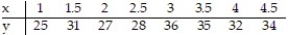 Summary statistics yield SSxx = 10.5, SSyy = 112, and SSxy = 25. Calculate the coefficient of determination rounded to the nearest ten-thousandth.
Summary statistics yield SSxx = 10.5, SSyy = 112, and SSxy = 25. Calculate the coefficient of determination rounded to the nearest ten-thousandth. سؤال
The coefficient of correlation between x and y is r = 0.59. Calculate the coefficient of determination  . Round
  to the nearest hundredth.
A) 0.59
B) 0.41
C) 0.65
D) 0.35
. Round to the nearest hundredth.A) 0.59
B) 0.41
C) 0.65
D) 0.35
سؤال
Analyze the residual lot below. Does it violate any of the conditions for an adequate linear model?
-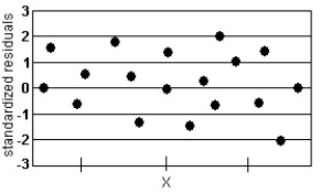
A) No, the plot of residuals is random.
B) Yes, the residuals do not display constant error variance.
C) Yes, there is a discernable pattern in the residuals.
-
A) No, the plot of residuals is random.
B) Yes, the residuals do not display constant error variance.
C) Yes, there is a discernable pattern in the residuals.

فتح الحزمة
قم بالتسجيل لفتح البطاقات في هذه المجموعة!
Unlock Deck
Unlock Deck
1/92
العب
ملء الشاشة (f)
Deck 4: Describing the Relation Between Two Variables
1
Construct a scatter diagram for the data.
-The data below are the temperatures on randomly chosen days during a summer class and the number of absences on those days.
-The data below are the temperatures on randomly chosen days during a summer class and the number of absences on those days.
2
Construct a scatter diagram for the data.
-The data below are the number of absences and the final grades of 9 randomly selected students from a literature class.
-The data below are the number of absences and the final grades of 9 randomly selected students from a literature class.
3
Construct a scatter diagram for the data.
-In order for employees of a company to work in a foreign office, they must take a test in the language of the country where they plan to work. The data below show the relationship between the number of years that employees have studied a particular language and the grades they received on the proficiency exam.
-In order for employees of a company to work in a foreign office, they must take a test in the language of the country where they plan to work. The data below show the relationship between the number of years that employees have studied a particular language and the grades they received on the proficiency exam.
4
Construct a scatter diagram for the data.
-Five brands of cigarettes were tested for the amounts of tar and nicotine they contained. All measurements are in milligrams per cigarette.
-Five brands of cigarettes were tested for the amounts of tar and nicotine they contained. All measurements are in milligrams per cigarette.
فتح الحزمة
افتح القفل للوصول البطاقات البالغ عددها 92 في هذه المجموعة.
فتح الحزمة
k this deck
5
Construct a scatter diagram for the data.
-The scores of nine members of a local community college women's golf team in two rounds of tournament play are listed below.
-The scores of nine members of a local community college women's golf team in two rounds of tournament play are listed below.
فتح الحزمة
افتح القفل للوصول البطاقات البالغ عددها 92 في هذه المجموعة.
فتح الحزمة
k this deck
6
Make a scatter diagram for the data. Use the scatter diagram to describe how, if at all, the variables are related.
-
A) The variables appear to be negatively, linearly related.
B) The variables appear to be positively, linearly related.
C) The variables do not appear to be linearly related.
D) The variables do not appear to be linearly related.
-
A) The variables appear to be negatively, linearly related.
B) The variables appear to be positively, linearly related.
C) The variables do not appear to be linearly related.
D) The variables do not appear to be linearly related.
فتح الحزمة
افتح القفل للوصول البطاقات البالغ عددها 92 في هذه المجموعة.
فتح الحزمة
k this deck
7
Make a scatter diagram for the data. Use the scatter diagram to describe how, if at all, the variables are related.
-
A) The variables do not appear to be linearly related.
B) The variables appear to be positively, linearly related.
C) The variables do not appear to be linearly related.
D) The variables appear to be negatively, linearly related.
-
A) The variables do not appear to be linearly related.
B) The variables appear to be positively, linearly related.
C) The variables do not appear to be linearly related.
D) The variables appear to be negatively, linearly related.
فتح الحزمة
افتح القفل للوصول البطاقات البالغ عددها 92 في هذه المجموعة.
فتح الحزمة
k this deck
8
Make a scatter diagram for the data. Use the scatter diagram to describe how, if at all, the variables are related.
-
A) The variables do not appear to be linearly related.
B) The variables appear to be positively, linearly related.
C) The variables do not appear to be linearly related.
D) The variables appear to be negatively, linearly related.
-
A) The variables do not appear to be linearly related.
B) The variables appear to be positively, linearly related.
C) The variables do not appear to be linearly related.
D) The variables appear to be negatively, linearly related.
فتح الحزمة
افتح القفل للوصول البطاقات البالغ عددها 92 في هذه المجموعة.
فتح الحزمة
k this deck
9
Use the scatter diagrams shown, labeled a through f to solve the problem.
-In which scatter diagram is r = 0.01?
A) d
B) c
C) e
D) f
-In which scatter diagram is r = 0.01?
A) d
B) c
C) e
D) f
فتح الحزمة
افتح القفل للوصول البطاقات البالغ عددها 92 في هذه المجموعة.
فتح الحزمة
k this deck
10
The data below represent the numbers of absences and the final grades of 15 randomly selected students from an astronomy class. Construct a scatter diagram for the data. Do you detect a trend?
فتح الحزمة
افتح القفل للوصول البطاقات البالغ عددها 92 في هذه المجموعة.
فتح الحزمة
k this deck
11
A medical researcher wishes to determine if there is a relationship between the number of prescriptions written by pediatricians and the ages of the children for whom the prescriptions are written. She surveys all the pediatricians in a geographical region to collect her data. What is the response variable?
A) Number of prescriptions written
B) Number of children for whom prescriptions were written
C) Pediatricians surveyed
D) Age of the children for whom prescriptions were written
A) Number of prescriptions written
B) Number of children for whom prescriptions were written
C) Pediatricians surveyed
D) Age of the children for whom prescriptions were written
فتح الحزمة
افتح القفل للوصول البطاقات البالغ عددها 92 في هذه المجموعة.
فتح الحزمة
k this deck
12
A history instructor has given the same pretest and the same final examination each semester. He is interested in determining if there is a relationship between the scores of the two tests. He computes the linear correlation coefficient and notes that it is 1.15. What does this correlation coefficient value tell the instructor?
A) The history instructor has made a computational error.
B) The correlation is something other than linear.
C) There is a strong negative correlation between the tests.
D) There is a strong positive correlation between the tests.
A) The history instructor has made a computational error.
B) The correlation is something other than linear.
C) There is a strong negative correlation between the tests.
D) There is a strong positive correlation between the tests.
فتح الحزمة
افتح القفل للوصول البطاقات البالغ عددها 92 في هذه المجموعة.
فتح الحزمة
k this deck
13
A traffic officer is compiling information about the relationship between the hour or the day and the speed over the limit at which the motorist is ticketed. He computes a correlation coefficient of 0.12. What does this tell the officer?
A) There is a moderate negative linear correlation.
B) There is insufficient evidence to make any conclusions about the relationship between the variables.
C) There is a weak positive linear correlation.
D) There is a moderate positive linear correlation.
A) There is a moderate negative linear correlation.
B) There is insufficient evidence to make any conclusions about the relationship between the variables.
C) There is a weak positive linear correlation.
D) There is a moderate positive linear correlation.
فتح الحزمة
افتح القفل للوصول البطاقات البالغ عددها 92 في هذه المجموعة.
فتح الحزمة
k this deck
14
Calculate the linear correlation coefficient for the data below.
A) 0.819
B) 0.990
C) 0.881
D) 0.792
A) 0.819
B) 0.990
C) 0.881
D) 0.792
فتح الحزمة
افتح القفل للوصول البطاقات البالغ عددها 92 في هذه المجموعة.
فتح الحزمة
k this deck
15
Calculate the linear correlation coefficient for the data below.
A) -0.885
B) -0.995
C) -0.671
D) -0.778
A) -0.885
B) -0.995
C) -0.671
D) -0.778
فتح الحزمة
افتح القفل للوصول البطاقات البالغ عددها 92 في هذه المجموعة.
فتح الحزمة
k this deck
16
Calculate the linear correlation coefficient for the data below.
A) -0.132
B) -0.549
C) -0.104
D) -0.581
A) -0.132
B) -0.549
C) -0.104
D) -0.581
فتح الحزمة
افتح القفل للوصول البطاقات البالغ عددها 92 في هذه المجموعة.
فتح الحزمة
k this deck
17
The data below are the ages and annual pharmacy b ills (in dollars) of 9 randomly selected employees. Calculate the linear correlation coefficient.
A) 0.908
B) 0.890
C) 0.960
D) 0.998
A) 0.908
B) 0.890
C) 0.960
D) 0.998
فتح الحزمة
افتح القفل للوصول البطاقات البالغ عددها 92 في هذه المجموعة.
فتح الحزمة
k this deck
18
Compute the linear correlation coefficient between the two variables and determine whether a linear relation exists.
-
A) r = 0.708; no linear relation exists
B) r = 0.235; no linear relation exists
C) r = 0.708; linear relation exists
D) r = -0.708; linear relation exists
-
A) r = 0.708; no linear relation exists
B) r = 0.235; no linear relation exists
C) r = 0.708; linear relation exists
D) r = -0.708; linear relation exists
فتح الحزمة
افتح القفل للوصول البطاقات البالغ عددها 92 في هذه المجموعة.
فتح الحزمة
k this deck
19
Compute the linear correlation coefficient between the two variables and determine whether a linear relation exists.
-
A) r = -0.335; no linear relation exists
B) r = -0.284; no linear relation exists
C) r = 0.462; linear relation exists
D) r = -0.335; linear relation exists
-
A) r = -0.335; no linear relation exists
B) r = -0.284; no linear relation exists
C) r = 0.462; linear relation exists
D) r = -0.335; linear relation exists
فتح الحزمة
افتح القفل للوصول البطاقات البالغ عددها 92 في هذه المجموعة.
فتح الحزمة
k this deck
20
Compute the linear correlation coefficient between the two variables and determine whether a linear relation exists.
-The table below shows the scores on an end-of-year project of 10 randomly selected architecture students and the number of days each student spent working on the project.
A) r = 0.847; linear relation exists
B) r = 0.761; no linear relation exists
C) r = 0.847; no linear relation exists
D) r = 0.761; linear relation exists
فتح الحزمة
افتح القفل للوصول البطاقات البالغ عددها 92 في هذه المجموعة.
فتح الحزمة
k this deck
21
Compute the linear correlation coefficient between the two variables and determine whether a linear relation exists.
-The table below shows the ages and weights (in pounds) of 9 randomly selected tennis coaches.
A) r = 0.908; linear relation exists
B) r = 0.960; no linear relation exists
C) r = 0.908; no linear relation exists
D) r = 0.960; linear relation exists
-The table below shows the ages and weights (in pounds) of 9 randomly selected tennis coaches.
A) r = 0.908; linear relation exists
B) r = 0.960; no linear relation exists
C) r = 0.908; no linear relation exists
D) r = 0.960; linear relation exists
فتح الحزمة
افتح القفل للوصول البطاقات البالغ عددها 92 في هذه المجموعة.
فتح الحزمة
k this deck
22
Compute the linear correlation coefficient between the two variables and determine whether a linear relation exists.
-To investigate the relationship between yield of soybeans and the amount of fertilizer used, a researcher divides a field into eight plots of equal size and applies a different amount of fertilizer to each plot. The table shows the yield of soybeans and the amount of fertilizer used for each plot.
A) r = 0.819; linear relation exists
B) r = 0.683; linear relation exists
C) r = 0.683; no linear relation exists
D) r = 0.729; no linear relation exists
فتح الحزمة
افتح القفل للوصول البطاقات البالغ عددها 92 في هذه المجموعة.
فتح الحزمة
k this deck
23
Find the equation of the regression line for the given data. Round values to the nearest thousandth.
A) =0.522x-2.097
B) =-0.552x+2.097
C) =2.097x-0.552
D) =2.097x+0.552
A)
=0.522x-2.097B)
=-0.552x+2.097C)
=2.097x-0.552D)
=2.097x+0.552 فتح الحزمة
افتح القفل للوصول البطاقات البالغ عددها 92 في هذه المجموعة.
فتح الحزمة
k this deck
24
Find the equation of the regression line for the given data. Round values to the nearest thousandth.
A) =-1.885x+0.758
B) =1.885x-0.758
C) =-0.758x-1.885
D) =0.758x+1.885
A)
=-1.885x+0.758B)
=1.885x-0.758C)
=-0.758x-1.885D)
=0.758x+1.885 فتح الحزمة
افتح القفل للوصول البطاقات البالغ عددها 92 في هذه المجموعة.
فتح الحزمة
k this deck
25
Find the equation of the regression line for the given data. Round values to the nearest thousandth.
A) =2.097x-0.206
B) =-0.206x+2.097
C) =0.206x-2.097
D) =-2.097x+0.206
A)
=2.097x-0.206B)
=-0.206x+2.097C)
=0.206x-2.097D)
=-2.097x+0.206 فتح الحزمة
افتح القفل للوصول البطاقات البالغ عددها 92 في هذه المجموعة.
فتح الحزمة
k this deck
26
The data below are the average one-way commute times (in minutes) for selected students and the number of absences for those students during the term. Find the equation of the regression line for the given data. What would be the predicted number of absences if the commute time was 95 minutes? Is this a reasonable question? Round the predicted number of absences to the nearest whole number. Round the regression line values to the nearest hundredth.
A) =0.45x-30.27; 12 absences; No, it is not reasonable. 95 minutes is well outside the scope of the model.
B) =0.45x+30.27; 73 absences; Yes, it is reasonable.
C) =0.45x+30.27; 73 absences; No, it is not reasonable. 95 minutes is well outside the scope of the model.
D) =0.45x-30.27; 12 absences; Yes, it is reasonable.
A)
=0.45x-30.27; 12 absences; No, it is not reasonable. 95 minutes is well outside the scope of the model.B)
=0.45x+30.27; 73 absences; Yes, it is reasonable.C)
=0.45x+30.27; 73 absences; No, it is not reasonable. 95 minutes is well outside the scope of the model.D)
=0.45x-30.27; 12 absences; Yes, it is reasonable. فتح الحزمة
افتح القفل للوصول البطاقات البالغ عددها 92 في هذه المجموعة.
فتح الحزمة
k this deck
27
The data below are the average one-way commute times (in minutes) for selected students and the number of absences for those students during the term. Find the equation of the regression line for the given data. What would be the predicted number of absences if the commute time was 40 minutes? Is this a reasonable question? Round the predicted number of absences to the nearest whole number. Round the regression line values to the nearest hundredth.
A) =0.45x+30.27; 48 absences; No, it is not reasonable. 40 minutes is well outside the scope of the model.
B) =0.45x-30.27;-12 absences; No, it is not reasonable. 40 minutes is well outside the scope of the model.
C) =0.45x+30.27; 48 absences; Yes, it is reasonable.
D) =0.45x-30.27;-12 absences; Yes, it is reasonable.
A)
=0.45x+30.27; 48 absences; No, it is not reasonable. 40 minutes is well outside the scope of the model.B)
=0.45x-30.27;-12 absences; No, it is not reasonable. 40 minutes is well outside the scope of the model.C)
=0.45x+30.27; 48 absences; Yes, it is reasonable.D)
=0.45x-30.27;-12 absences; Yes, it is reasonable. فتح الحزمة
افتح القفل للوصول البطاقات البالغ عددها 92 في هذه المجموعة.
فتح الحزمة
k this deck
28
The data below are the number of absences and the final grades of 9 randomly selected students from a literature class. Find the equation of the regression line for the given data. What would be the predicted final grade if a student was absent 14 times? Round the regression line values to the nearest hundredth. Round the predicted grade to the nearest whole number.
A) =96.14x-2.75; 1343
B) =-2.75x-96.14; 134.64
C) =-96.14x+2.75; 1343
D) =-2.75x+96.14; 58
A)
=96.14x-2.75; 1343B)
=-2.75x-96.14; 134.64C)
=-96.14x+2.75; 1343D)
=-2.75x+96.14; 58 فتح الحزمة
افتح القفل للوصول البطاقات البالغ عددها 92 في هذه المجموعة.
فتح الحزمة
k this deck
29
A manager wishes to determine the relationship between the number of miles traveled (in hundreds of miles) by her sales representatives and their amount of sales (in thousands of dollars) per month. Find the equation of the regression line for the given data. What would be the predicted sales if the sales representative traveled 0 miles? Is this reasonable? Why or why not? Round the regression line values to the nearest hundredth.
A) =3.53x+37.92; $37,920; Yes, it is reasonable.
B) =3.53x+37.92; $3792; No; it is not reasonable for a representative to travel 0 miles and have a positive amount of sales.
C) =37.92x+3.53; $3792; Yes, it is reasonable.
D) =3.53x+37.92; $37,920; No; it is not reasonable for a representative to travel 0 miles and have a positive amount of sales.
A)
=3.53x+37.92; $37,920; Yes, it is reasonable.B)
=3.53x+37.92; $3792; No; it is not reasonable for a representative to travel 0 miles and have a positive amount of sales.C)
=37.92x+3.53; $3792; Yes, it is reasonable.D)
=3.53x+37.92; $37,920; No; it is not reasonable for a representative to travel 0 miles and have a positive amount of sales. فتح الحزمة
افتح القفل للوصول البطاقات البالغ عددها 92 في هذه المجموعة.
فتح الحزمة
k this deck
30
A manager wishes to determine the relationship between the number of years her sales representatives have been employed by the firm and their amount of sales (in thousands of dollars) per month. Find the equation of the regression line for the given data. What would be the predicted sales if the sales representative was employed by the firm for 30 years Is this reasonable? Why or why not? Round the regression line values to the nearest hundredth.
A) =3.53x+37.92; $143,820;; Yes, it is reasonable.
B) =3.53x-37.92; $67,980; No; it is not reasonable. 30 years of employment is well outside the scope of the model.
C) =3.53x-37.92; $67,980; Yes; it is reasonable.
D) =3.53x+37.92; $143,820; No; it is not reasonable. 30 years of employment is well outside the scope of the model.
A)
=3.53x+37.92; $143,820;; Yes, it is reasonable.B)
=3.53x-37.92; $67,980; No; it is not reasonable. 30 years of employment is well outside the scope of the model.C)
=3.53x-37.92; $67,980; Yes; it is reasonable.D)
=3.53x+37.92; $143,820; No; it is not reasonable. 30 years of employment is well outside the scope of the model. فتح الحزمة
افتح القفل للوصول البطاقات البالغ عددها 92 في هذه المجموعة.
فتح الحزمة
k this deck
31
The table shows, for the years 1997-2012, the mean hourly wage for residents of the town of Pity Me and the mean weekly rent paid by the residents. Summary statistics yield: = 1222.2771, = 3031.7125, = 9144.9375, = 21.2675, and Find the least squares line that uses mean hourly wage to predict mean weekly rent. Round values to the nearest ten-thousandth.
Summary statistics yield: = 1222.2771, = 3031.7125, = 9144.9375, = 21.2675, and Find the least squares line that uses mean hourly wage to predict mean weekly rent. Round values to the nearest ten-thousandth. فتح الحزمة
افتح القفل للوصول البطاقات البالغ عددها 92 في هذه المجموعة.
فتح الحزمة
k this deck
32
A county real estate appraiser wants to develop a statistical model to predict the appraised value of houses in a section of the county called East Meadow. One of the many variables thought to be an important predictor of appraised value is the number of rooms in the house. Consequently, the appraiser decided to fit the simple linear regression model, where y = appraised value of the house (in $thousands) and x = number of rooms. Using data collected for a sample of n= 74 houses in East Meadow, the following results were obtained: Give a practical interpretation of the estimate of the slope of the least squares line.
A) For each additional room in the house, we estimate the appraised value to increase $ 17, 890.
B) For each additional dollar of appraised value, we estimate the number of rooms in the house to increase by 17. 89 rooms.
C) For each additional room in the house, we estimate the appraised value to increase $74,800.
D) For a house with 0 rooms, we estimate the appraised value to be $74,800.
where y = appraised value of the house (in $thousands) and x = number of rooms. Using data collected for a sample of n= 74 houses in East Meadow, the following results were obtained: Give a practical interpretation of the estimate of the slope of the least squares line.A) For each additional room in the house, we estimate the appraised value to increase $ 17, 890.
B) For each additional dollar of appraised value, we estimate the number of rooms in the house to increase by 17. 89 rooms.
C) For each additional room in the house, we estimate the appraised value to increase $74,800.
D) For a house with 0 rooms, we estimate the appraised value to be $74,800.
فتح الحزمة
افتح القفل للوصول البطاقات البالغ عددها 92 في هذه المجموعة.
فتح الحزمة
k this deck
33
A county real estate appraiser wants to develop a statistical model to predict the appraised value of houses in a section of the county called East Meadow. One of the many variables thought to be an important predictor of appraised value is the number of rooms in the house. Consequently, the appraiser decided to fit the simple linear regression model, where y = appraised value of the house (in $thousands) and x = number of rooms. Using data collected for a sample of n= 74 houses in East Meadow, the following results were obtained: Give a practical interpretation of the estimate of the y-intercept of the least squares line.
A) For each additional room in the house, we estimate the appraised value to increase $19,720.
B) For each additional room in the house, we estimate the appraised value to increase $74,800.
C) There is no practical interpretation, since a house with 0 rooms is nonsensical.
D) We estimate the base appraised value for any house to be $74,800.
where y = appraised value of the house (in $thousands) and x = number of rooms. Using data collected for a sample of n= 74 houses in East Meadow, the following results were obtained: Give a practical interpretation of the estimate of the y-intercept of the least squares line.A) For each additional room in the house, we estimate the appraised value to increase $19,720.
B) For each additional room in the house, we estimate the appraised value to increase $74,800.
C) There is no practical interpretation, since a house with 0 rooms is nonsensical.
D) We estimate the base appraised value for any house to be $74,800.
فتح الحزمة
افتح القفل للوصول البطاقات البالغ عددها 92 في هذه المجموعة.
فتح الحزمة
k this deck
34
Is there a relationship between the raises administrators at State University receive and their performance on the job? A faculty group wants to determine whether job rating (x) is a useful linear predictor of raise (y). Consequently, the group considered the straight-line regression model, Using the method of least squares, the faculty group obtained the following prediction equation, Interpret the estimated slope of the line.
A) For a $1 increase in an administrator's raise, we estimate the administrator's rating to decrease 2,000 points.
B) For a 1-point increase in an administrator's rating, we estimate the administrator's raise to decrease $2,000.
C) For a 1-point increase in an administrator's rating, we estimate the administrator's raise to increase $2,000.
D) For an administrator with a rating of 1.0, we estimate his/her raise to be $2,000.
Using the method of least squares, the faculty group obtained the following prediction equation, Interpret the estimated slope of the line.A) For a $1 increase in an administrator's raise, we estimate the administrator's rating to decrease 2,000 points.
B) For a 1-point increase in an administrator's rating, we estimate the administrator's raise to decrease $2,000.
C) For a 1-point increase in an administrator's rating, we estimate the administrator's raise to increase $2,000.
D) For an administrator with a rating of 1.0, we estimate his/her raise to be $2,000.
فتح الحزمة
افتح القفل للوصول البطاقات البالغ عددها 92 في هذه المجموعة.
فتح الحزمة
k this deck
35
Is there a relationship between the raises administrators at State University receive and their performance on the job? A faculty group wants to determine whether job rating (x) is a useful linear predictor of raise (y). Consequently, the group considered the straight-line regression model, Using the method of least squares, the faculty group obtained the following prediction equation, Interpret the estimated y-intercept of the line.
A) The base administrator raise at State University is $14,000.
B) For a 1-point increase in an administrator's rating, we estimate the administrator's raise to increase $14,000.
C) There is no practical interpretation, since rating of 0 is nonsensical and outside the range of the sample data.
D) For an administrator who receives a rating of zero, we estimate his or her raise to be $14,000.
Using the method of least squares, the faculty group obtained the following prediction equation, Interpret the estimated y-intercept of the line.A) The base administrator raise at State University is $14,000.
B) For a 1-point increase in an administrator's rating, we estimate the administrator's raise to increase $14,000.
C) There is no practical interpretation, since rating of 0 is nonsensical and outside the range of the sample data.
D) For an administrator who receives a rating of zero, we estimate his or her raise to be $14,000.
فتح الحزمة
افتح القفل للوصول البطاقات البالغ عددها 92 في هذه المجموعة.
فتح الحزمة
k this deck
36
A large national bank charges local companies for using its services. A bank official reported the results of a regression analysis designed to predict the bank's charges (y), measured in dollars per month, for services rendered to local companies. One independent variable used to predict service charge to a company is the company's sales revenue (x), measured in millions of dollars. Data for 21 companies who use the bank's services were used to fit the model, The results of the simple linear regression are provided below. = 2,700 + 20x, s = 65, 2-tailed p-value = 0.064 (for testing )Interpret the estimate of , the y-intercept of the line.
A) All companies will be charged at least $2,700 by the bank.
B) About 95% of the observed service charges fall within $2,700 of the least squares line.
C) There is no practical interpretation since a sales revenue of $0 is a nonsensical value.
D) For every $1 million increase in sales revenue, we expect a service charge to increase $2,700.
The results of the simple linear regression are provided below. = 2,700 + 20x, s = 65, 2-tailed p-value = 0.064 (for testing )Interpret the estimate of , the y-intercept of the line.A) All companies will be charged at least $2,700 by the bank.
B) About 95% of the observed service charges fall within $2,700 of the least squares line.
C) There is no practical interpretation since a sales revenue of $0 is a nonsensical value.
D) For every $1 million increase in sales revenue, we expect a service charge to increase $2,700.
فتح الحزمة
افتح القفل للوصول البطاقات البالغ عددها 92 في هذه المجموعة.
فتح الحزمة
k this deck
37
Civil engineers often use the straight-line equation, = + x, to model the relationship between the mean shear strength of masonry joints and precompression stress, x. To test this theory, a series of stress tests were performed on solid bricks arranged in triplets and joined with mortar. The precompression stress was varied for each triplet and the ultimate shear load just before failure (called the shear strength) was recorded. The stress results for n = 7 triplet tests is shown in the accompanying table followed by a SAS printout of the regression analysis.
-Give a practical interpretation of the estimate of the slope of the least squares line.
A) For a triplet test with a precompression stress of 1 ton, we estimate the shear strength of the joint to be 0.987 ton.
B) For every 0.987 ton increase in precompression stress, we estimate the shear strength of the joint to increase by 1 ton.
C) For a triplet test with a precompression stress of 0 tons, we estimate the shear strength of the joint to be 1.19 tons.
D) For every 1 ton increase in precompression stress, we estimate the shear strength of the joint to increase by 0.987 ton.
= + x, to model the relationship between the mean shear strength of masonry joints and precompression stress, x. To test this theory, a series of stress tests were performed on solid bricks arranged in triplets and joined with mortar. The precompression stress was varied for each triplet and the ultimate shear load just before failure (called the shear strength) was recorded. The stress results for n = 7 triplet tests is shown in the accompanying table followed by a SAS printout of the regression analysis. -Give a practical interpretation of the estimate of the slope of the least squares line.
A) For a triplet test with a precompression stress of 1 ton, we estimate the shear strength of the joint to be 0.987 ton.
B) For every 0.987 ton increase in precompression stress, we estimate the shear strength of the joint to increase by 1 ton.
C) For a triplet test with a precompression stress of 0 tons, we estimate the shear strength of the joint to be 1.19 tons.
D) For every 1 ton increase in precompression stress, we estimate the shear strength of the joint to increase by 0.987 ton.
فتح الحزمة
افتح القفل للوصول البطاقات البالغ عددها 92 في هذه المجموعة.
فتح الحزمة
k this deck
38
Civil engineers often use the straight-line equation, = + x, to model the relationship between the mean shear strength of masonry joints and precompression stress, x. To test this theory, a series of stress tests were performed on solid bricks arranged in triplets and joined with mortar. The precompression stress was varied for each triplet and the ultimate shear load just before failure (called the shear strength) was recorded. The stress results for n = 7 triplet tests is shown in the accompanying table followed by a SAS printout of the regression analysis.
- Give a practical interpretation of the estimate of the y-intercept of the least squares line.
A) For a triplet test with a precompression stress of 0 tons, we estimate the shear strength of the joint to increase 1.19 tons.
B) There is no practical interpretation since a triplet test with a precompression stress of 0 tons is outside the range of the sample data.
C) For a triplet test with a precompression stress of 0 tons, we estimate the shear strength of the joint to be 1.19 tons.
D) For every 1 ton increase in precompression stress, we estimate the shear strength of the joint to increase by 0.987 ton.
= + x, to model the relationship between the mean shear strength of masonry joints and precompression stress, x. To test this theory, a series of stress tests were performed on solid bricks arranged in triplets and joined with mortar. The precompression stress was varied for each triplet and the ultimate shear load just before failure (called the shear strength) was recorded. The stress results for n = 7 triplet tests is shown in the accompanying table followed by a SAS printout of the regression analysis. - Give a practical interpretation of the estimate of the y-intercept of the least squares line.
A) For a triplet test with a precompression stress of 0 tons, we estimate the shear strength of the joint to increase 1.19 tons.
B) There is no practical interpretation since a triplet test with a precompression stress of 0 tons is outside the range of the sample data.
C) For a triplet test with a precompression stress of 0 tons, we estimate the shear strength of the joint to be 1.19 tons.
D) For every 1 ton increase in precompression stress, we estimate the shear strength of the joint to increase by 0.987 ton.
فتح الحزمة
افتح القفل للوصول البطاقات البالغ عددها 92 في هذه المجموعة.
فتح الحزمة
k this deck
39
Each year a nationally recognized publication conducts its "Survey of America's Best Graduate and Professional Schools." An academic advisor wants to predict the typical starting salary of a graduate at a top business school using GMAT score of the school as a predictor variable. Total GMAT scores range from 200 to 800. A simple linear regression of SALARY versus GMAT using 25 data points shown below.
-Give a practical interpretation of = -92040.
A) We expect to predict SALARY to within 2(92040) = $184,080 of its true value using GMAT in a straight-line model.
B) We estimate the base SALARY of graduates of a top business school to be $-92,040.
C) We estimate SALARY to decrease $92,040 for every 1-point increase in GMAT.
D) The value has no practical interpretation since a GMAT of 0 is nonsensical and outside the range of the sample data.
-Give a practical interpretation of
= -92040.A) We expect to predict SALARY to within 2(92040) = $184,080 of its true value using GMAT in a straight-line model.
B) We estimate the base SALARY of graduates of a top business school to be $-92,040.
C) We estimate SALARY to decrease $92,040 for every 1-point increase in GMAT.
D) The value has no practical interpretation since a GMAT of 0 is nonsensical and outside the range of the sample data.
فتح الحزمة
افتح القفل للوصول البطاقات البالغ عددها 92 في هذه المجموعة.
فتح الحزمة
k this deck
40
Each year a nationally recognized publication conducts its "Survey of America's Best Graduate and Professional Schools." An academic advisor wants to predict the typical starting salary of a graduate at a top business school using GMAT score of the school as a predictor variable. Total GMAT scores range from 200 to 800. A simple linear regression of SALARY versus GMAT using 25 data points shown below.
-Give a practical interpretation of = 228.
A) We expect to predict SALARY to within 2(228) = $456 of its true value using GMAT in a straight-line model.
B) The value has no practical interpretation since a GMAT of 0 is nonsensical and outside the range of the sample data.
C) We estimate SALARY to increase $228 for every 1-point increase in GMAT.
D) We estimate GMAT to increase 228 points for every $1 increase in SALARY.
-Give a practical interpretation of
= 228.A) We expect to predict SALARY to within 2(228) = $456 of its true value using GMAT in a straight-line model.
B) The value has no practical interpretation since a GMAT of 0 is nonsensical and outside the range of the sample data.
C) We estimate SALARY to increase $228 for every 1-point increase in GMAT.
D) We estimate GMAT to increase 228 points for every $1 increase in SALARY.
فتح الحزمة
افتح القفل للوصول البطاقات البالغ عددها 92 في هذه المجموعة.
فتح الحزمة
k this deck
41
A real estate magazine reported the results of a regression analysis designed to predict the price (y), measured in dollars, of residential properties recently sold in a northern Virginia subdivision. One independent variable used to predict sale price is GLA, gross living area (x), measured in square feet. Data for 157 properties were used to fit the model, = + x. The results of the simple linear regression are provided below. Interpret the estimate of , the y-intercept of the line.
A) For every 1-sq ft. increase in GLA, we expect a property's sale price to increase $96,600.
B) About 95% of the observed sale prices fall within $96,600 of the least squares line.
C) There is no practical interpretation, since a gross living area of 0 is a nonsensical value.
D) All residential properties in Virginia will sell for at least $96,600.
= + x. The results of the simple linear regression are provided below. Interpret the estimate of , the y-intercept of the line.A) For every 1-sq ft. increase in GLA, we expect a property's sale price to increase $96,600.
B) About 95% of the observed sale prices fall within $96,600 of the least squares line.
C) There is no practical interpretation, since a gross living area of 0 is a nonsensical value.
D) All residential properties in Virginia will sell for at least $96,600.
فتح الحزمة
افتح القفل للوصول البطاقات البالغ عددها 92 في هذه المجموعة.
فتح الحزمة
k this deck
42
In a comprehensive road test on all new car models, one variable measured is the time it takes a car to accelerate from 0 to 60 miles per hour. To model acceleration time, a regression analysis is conducted on a random sample of 129 new cars.
TIME60: y = Elapsed time (in seconds) from 0 mph to 60 mph
MAX: = Maximum speed attained (miles per hour)
Initially, the simple linear model E(y) = + was fit to the data. Computer printouts for the analysis are given below: Find and interpret the estimate in the printout above.
TIME60: y = Elapsed time (in seconds) from 0 mph to 60 mph
MAX:
= Maximum speed attained (miles per hour)Initially, the simple linear model E(y) =
+ was fit to the data. Computer printouts for the analysis are given below: Find and interpret the estimate in the printout above. فتح الحزمة
افتح القفل للوصول البطاقات البالغ عددها 92 في هذه المجموعة.
فتح الحزمة
k this deck
43
In a study of feeding behavior, zoologists recorded the number of grunts of a warthog feeding by a lake in the 15 minute period following the addition of food. The data showing the weekly number of grunts and the age of the warthog (in days) are listed below: a. Write the equation of a straight-line model relating number of grunts (y) to age (x).
b. Give the least squares prediction equation.
c. Give a practical interpretation of the value of if possible.
d. Give a practical interpretation of the value of if possible.
a. Write the equation of a straight-line model relating number of grunts (y) to age (x).b. Give the least squares prediction equation.
c. Give a practical interpretation of the value of
if possible.d. Give a practical interpretation of the value of
if possible. فتح الحزمة
افتح القفل للوصول البطاقات البالغ عددها 92 في هذه المجموعة.
فتح الحزمة
k this deck
44
Given the equation of a regression line is = -5.5x - 0.7, what is the best predicted value for y given x= 7.4?
A) 40.00
B) 41.40
C) -41.40
D) -40.00
= -5.5x - 0.7, what is the best predicted value for y given x= 7.4?A) 40.00
B) 41.40
C) -41.40
D) -40.00
فتح الحزمة
افتح القفل للوصول البطاقات البالغ عددها 92 في هذه المجموعة.
فتح الحزمة
k this deck
45
Use the regression equation to predict the value of y for x = -3.4.
A) -7.682
B) 3.974
C) 0.220
D) -6.578
A) -7.682
B) 3.974
C) 0.220
D) -6.578
فتح الحزمة
افتح القفل للوصول البطاقات البالغ عددها 92 في هذه المجموعة.
فتح الحزمة
k this deck
46
Use the regression equation to predict the value of y for x = -1.1.
A) 1.051
B) -2.719
C) -1.315
D) 2.832
A) 1.051
B) -2.719
C) -1.315
D) 2.832
فتح الحزمة
افتح القفل للوصول البطاقات البالغ عددها 92 في هذه المجموعة.
فتح الحزمة
k this deck
47
In an area of the Great Plains, records were kept on the relationship between the rainfall (in inches) and the yield of wheat (bushels per acre). Which is the best predicted value for y given x = 18.1?
A) 83.3
B) 83.5
C) 84.0
D) 83.8
A) 83.3
B) 83.5
C) 84.0
D) 83.8
فتح الحزمة
افتح القفل للوصول البطاقات البالغ عددها 92 في هذه المجموعة.
فتح الحزمة
k this deck
48
A calculus instructor is interested in finding the strength of a relationship between the final exam grades of students enrolled in Calculus I and Calculus II at his college. The data (in percentages) are listed below. a) Graph a scatter diagram of the data.
b) Find an equation of the regression line.
c) Predict a Calculus II exam score for a student who receives an 80 in Calculus I.
a) Graph a scatter diagram of the data.b) Find an equation of the regression line.
c) Predict a Calculus II exam score for a student who receives an 80 in Calculus I.
فتح الحزمة
افتح القفل للوصول البطاقات البالغ عددها 92 في هذه المجموعة.
فتح الحزمة
k this deck
49
In one area of Russia, records were kept on the relationship between the rainfall (in inches) and the yield of wheat (bushels per acre). The data for a 9 year period is as follows: The equation of the line of least squares is given as = -9.12 + 4.38x.
-How many bushels of wheat per acre can be predicted if it is expected that there will be 17 inches of rain?
A) 5.96
B) 61.18
C) 65.34
D) 52.06
The equation of the line of least squares is given as = -9.12 + 4.38x. -How many bushels of wheat per acre can be predicted if it is expected that there will be 17 inches of rain?
A) 5.96
B) 61.18
C) 65.34
D) 52.06
فتح الحزمة
افتح القفل للوصول البطاقات البالغ عددها 92 في هذه المجموعة.
فتح الحزمة
k this deck
50
In an area of Russia, records were kept on the relationship between the rainfall (in inches) and the yield of wheat (bushels per acre). The data for a 9 year period is as follows: The equation of the line of least squares is given as = -9.12 + 4.38x.
-What would be the expected number of inches of rain if the yield is 60 bushels of wheat per acre?
A) 64.74
B) 253.68
C) 11.62
D) 15.78
The equation of the line of least squares is given as = -9.12 + 4.38x. -What would be the expected number of inches of rain if the yield is 60 bushels of wheat per acre?
A) 64.74
B) 253.68
C) 11.62
D) 15.78
فتح الحزمة
افتح القفل للوصول البطاقات البالغ عددها 92 في هذه المجموعة.
فتح الحزمة
k this deck
51
In an area of Russia, records were kept on the relationship between the rainfall (in inches) and the yield of wheat (bushels per acre). The data for a 9 year period is as follows: The equation of the line of least squares is given as = -9.12 + 4.38x.
- How many bushels of wheat per acre can be predicted if it is expected that there will be 30 inches of rain?
A) Cannot be certain of the result because 30 inches of rain exceeds the observed data.
B) 8.93
C) 122.28
D) 140.52
The equation of the line of least squares is given as = -9.12 + 4.38x.- How many bushels of wheat per acre can be predicted if it is expected that there will be 30 inches of rain?
A) Cannot be certain of the result because 30 inches of rain exceeds the observed data.
B) 8.93
C) 122.28
D) 140.52
فتح الحزمة
افتح القفل للوصول البطاقات البالغ عددها 92 في هذه المجموعة.
فتح الحزمة
k this deck
52
The regression line for the given data is = 2.097x - 0.552. Determine the residual of a data point for which x = 3 and y = 6.
A) 5.739
B) -9.03
C) 11.739
D) 0.261
= 2.097x - 0.552. Determine the residual of a data point for which x = 3 and y = 6. A) 5.739
B) -9.03
C) 11.739
D) 0.261
فتح الحزمة
افتح القفل للوصول البطاقات البالغ عددها 92 في هذه المجموعة.
فتح الحزمة
k this deck
53
The regression line for the given data is = -1.885x + 0.758. Determine the residual of a data point for which x = 4 and y = -6.
A) -12.782
B) -8.068
C) 0.782
D) -6.782
= -1.885x + 0.758. Determine the residual of a data point for which x = 4 and y = -6. A) -12.782
B) -8.068
C) 0.782
D) -6.782
فتح الحزمة
افتح القفل للوصول البطاقات البالغ عددها 92 في هذه المجموعة.
فتح الحزمة
k this deck
54
The regression line for the given data is = -0.206x + 2.097. Determine the residual of a data point for which x = 0 and y = 5.
A) 2.097
B) 7.097
C) 2.903
D) -1.067
= -0.206x + 2.097. Determine the residual of a data point for which x = 0 and y = 5. A) 2.097
B) 7.097
C) 2.903
D) -1.067
فتح الحزمة
افتح القفل للوصول البطاقات البالغ عددها 92 في هذه المجموعة.
فتح الحزمة
k this deck
55
The regression line for the given data is = 5.044x + 56.11. Determine the residual of a data point for which x = 4 and y = 78.
A) 154.286
B) 76.286
C) -445.542
D) 1.714
= 5.044x + 56.11. Determine the residual of a data point for which x = 4 and y = 78. A) 154.286
B) 76.286
C) -445.542
D) 1.714
فتح الحزمة
افتح القفل للوصول البطاقات البالغ عددها 92 في هذه المجموعة.
فتح الحزمة
k this deck
56
The regression line for the given data is = 0.449x - 30.27. Determine the residual of a data point for which x = 100 and y = 15.
A) 14.63
B) 0.37
C) 29.63
D) 123.535
= 0.449x - 30.27. Determine the residual of a data point for which x = 100 and y = 15. A) 14.63
B) 0.37
C) 29.63
D) 123.535
فتح الحزمة
افتح القفل للوصول البطاقات البالغ عددها 92 في هذه المجموعة.
فتح الحزمة
k this deck
57
The regression line for the given data is = 1.488x + 60.46. Determine the residual of a data point for which x = 41 and y = 120.
A) -1.468
B) -198.02
C) 241.468
D) 121.468
= 1.488x + 60.46. Determine the residual of a data point for which x = 41 and y = 120. A) -1.468
B) -198.02
C) 241.468
D) 121.468
فتح الحزمة
افتح القفل للوصول البطاقات البالغ عددها 92 في هذه المجموعة.
فتح الحزمة
k this deck
58
The regression line for the given data is = -2.75x + 96.14. Determine the residual of a data point for which x = 0 and y = 98.
A) 173.36
B) 96.14
C) 194.14
D) 1.86
= -2.75x + 96.14. Determine the residual of a data point for which x = 0 and y = 98. A) 173.36
B) 96.14
C) 194.14
D) 1.86
فتح الحزمة
افتح القفل للوصول البطاقات البالغ عددها 92 في هذه المجموعة.
فتح الحزمة
k this deck
59
The regression line for the given data is = 3.53x + 37.92. Determine the residual of a data point for which x = 8 and y = 65.
A) 66.16
B) 131.16
C) -259.37
D) -1.16
= 3.53x + 37.92. Determine the residual of a data point for which x = 8 and y = 65. A) 66.16
B) 131.16
C) -259.37
D) -1.16
فتح الحزمة
افتح القفل للوصول البطاقات البالغ عددها 92 في هذه المجموعة.
فتح الحزمة
k this deck
60
The regression line for the given data is = 6.91x + 46.26. Determine the residual of a data point for which x = 2 and y = 58.
A) 118.08
B) -2.08
C) 60.08
D) -445.04
= 6.91x + 46.26. Determine the residual of a data point for which x = 2 and y = 58. A) 118.08
B) -2.08
C) 60.08
D) -445.04
فتح الحزمة
افتح القفل للوصول البطاقات البالغ عددها 92 في هذه المجموعة.
فتح الحزمة
k this deck
61
The regression line for the given data is = 4.379x + 4.267. Determine the residual of a data point for which x = 10.5 and y = 50.5.
A) 50.2465
B) 100.7465
C) 0.2535
D) -214.9065
= 4.379x + 4.267. Determine the residual of a data point for which x = 10.5 and y = 50.5. A) 50.2465
B) 100.7465
C) 0.2535
D) -214.9065
فتح الحزمة
افتح القفل للوصول البطاقات البالغ عددها 92 في هذه المجموعة.
فتح الحزمة
k this deck
62
Compute the sum of the squared residuals of the least-squares line for the given data.
A) 0
B) 2.097
C) 7.624
D) 1.036
A) 0
B) 2.097
C) 7.624
D) 1.036
فتح الحزمة
افتح القفل للوصول البطاقات البالغ عددها 92 في هذه المجموعة.
فتح الحزمة
k this deck
63
In a study of feeding behavior, zoologists recorded the number of grunts of a warthog feeding by a lake in a 15 minute time period following the addition of food. The data showing the weekly number of grunts and the age of the warthog (in days) are listed below. Compute the sum of the squared residuals of the least squared line for the given data.
A) 13.74
B) 188.84
C) 74.39
D) 5533.53
A) 13.74
B) 188.84
C) 74.39
D) 5533.53
فتح الحزمة
افتح القفل للوصول البطاقات البالغ عددها 92 في هذه المجموعة.
فتح الحزمة
k this deck
64
The data below are the ages and systolic blood pressure (measured in Millimeters of mercury) of 9 randomly selected adults.
A) 123.63
B) 1.41
C) 11.11
D) 1.99
A) 123.63
B) 1.41
C) 11.11
D) 1.99
فتح الحزمة
افتح القفل للوصول البطاقات البالغ عددها 92 في هذه المجموعة.
فتح الحزمة
k this deck
65
Choose the coefficient of determination that matches the scatterplot. Assume that the scales on the horizontal and vertical axes are the same.
-
A) =0.96
B) =0.77
C) =0.38
D) =0.51
-
A)
=0.96B)
=0.77C)
=0.38D)
=0.51 فتح الحزمة
افتح القفل للوصول البطاقات البالغ عددها 92 في هذه المجموعة.
فتح الحزمة
k this deck
66
Choose the coefficient of determination that matches the scatterplot. Assume that the scales on the horizontal and vertical axes are the same.
-
A) =0.12
B) =0.82
C) =0.43
D) =-0.43
-
A)
=0.12B)
=0.82C)
=0.43D)
=-0.43 فتح الحزمة
افتح القفل للوصول البطاقات البالغ عددها 92 في هذه المجموعة.
فتح الحزمة
k this deck
67
Choose the coefficient of determination that matches the scatterplot. Assume that the scales on the horizontal and vertical axes are the same.
-
A) =0.76
B) =0.41
C) =-0.31
D) =0.097
-
A)
=0.76B)
=0.41C)
=-0.31D)
=0.097 فتح الحزمة
افتح القفل للوصول البطاقات البالغ عددها 92 في هذه المجموعة.
فتح الحزمة
k this deck
68
Use the linear correlation coefficient given to determine the coefficient of determination ,
-r = 0.32
A) =56.57%
B) =5.66%
C) =10.24%
D) =1.024%
-r = 0.32
A)
=56.57%B)
=5.66%C)
=10.24%D)
=1.024% فتح الحزمة
افتح القفل للوصول البطاقات البالغ عددها 92 في هذه المجموعة.
فتح الحزمة
k this deck
69
Use the linear correlation coefficient given to determine the coefficient of determination ,
-r = -0.42
A) =-17.64%
B) =17.64%
C) =-64.81%
D) =64.81%
-r = -0.42
A)
=-17.64%B)
=17.64%C)
=-64.81%D)
=64.81% فتح الحزمة
افتح القفل للوصول البطاقات البالغ عددها 92 في هذه المجموعة.
فتح الحزمة
k this deck
70
In a study of feeding behavior, zoologists recorded the number of grunts of a warthog feeding by a lake in the 15 minute period following the addition of food. The data showing the weekly number of grunts and the age of the warthog (in days) are listed below. Find and interpret the value of . Round to the nearest thousandth.
. Round to the nearest thousandth. فتح الحزمة
افتح القفل للوصول البطاقات البالغ عددها 92 في هذه المجموعة.
فتح الحزمة
k this deck
71
In a comprehensive road test on all new car models, one variable measured is the time it takes a car to accelerate from 0 to 60 miles per hour. To model acceleration time, a regression analysis is conducted on a random sample of 129 new cars. Approximately what percentage, rounded to the nearest whole percent, of the sample variation in acceleration time can be explained by the simple linear model?
A) 8%
B) 70%
C) -17%
D) 0%
Approximately what percentage, rounded to the nearest whole percent, of the sample variation in acceleration time can be explained by the simple linear model?A) 8%
B) 70%
C) -17%
D) 0%
فتح الحزمة
افتح القفل للوصول البطاقات البالغ عددها 92 في هذه المجموعة.
فتح الحزمة
k this deck
72
A manufacturer of boiler drums wants to use regression to predict the number of man-hours needed to erect drums in the future. The manufacturer collected a random sample of 35 boilers and measured the following two variables: Give a practical interpretation of the coefficient of determination, . Express to the nearest whole percent.
A) About 43% of the sample variation in number of man-hours can be explained by the simple linear model.
B) About 2.06% of the sample variation in number of man-hours can be explained by the simple linear model.
C) Man hours needed to erect drums will be associated with boiler design pressure 43% of the time.
D) =1.88+0.00321x will be correct 43% of the time.
Give a practical interpretation of the coefficient of determination, . Express to the nearest whole percent.A) About 43% of the sample variation in number of man-hours can be explained by the simple linear model.
B) About 2.06% of the sample variation in number of man-hours can be explained by the simple linear model.
C) Man hours needed to erect drums will be associated with boiler design pressure 43% of the time.
D)
=1.88+0.00321x will be correct 43% of the time. فتح الحزمة
افتح القفل للوصول البطاقات البالغ عددها 92 في هذه المجموعة.
فتح الحزمة
k this deck
73
Civil engineers often use the straight-line equation, E(y) = + x, to model the relationship between the mean shear strength E(y) of masonry joints and precompression stress, x. To test this theory, a series of stress tests were performed on solid bricks arranged in triplets and joined with mortar. The precompression stress was varied for each triplet and the ultimate shear load just before failure (called the shear strength) was recorded. The stress results for n = 7 triplet tests is shown in the accompanying table followed by a SAS printout of the regression analysis.
A) In repeated sampling, approximately 91% of all similarly constructed regression lines will accurately predict shear strength.
B) About 91% of the total variation in the sample of y-values can be explained by (or attributed to) the linear relationship between shear strength and precompression stress.
C) We expect about 91% of the observed shear strength values to lie on the least squares line.
D) We expect to predict the shear strength of a triplet test to within about .91 ton of its true value.
+ x, to model the relationship between the mean shear strength E(y) of masonry joints and precompression stress, x. To test this theory, a series of stress tests were performed on solid bricks arranged in triplets and joined with mortar. The precompression stress was varied for each triplet and the ultimate shear load just before failure (called the shear strength) was recorded. The stress results for n = 7 triplet tests is shown in the accompanying table followed by a SAS printout of the regression analysis. A) In repeated sampling, approximately 91% of all similarly constructed regression lines will accurately predict shear strength.
B) About 91% of the total variation in the sample of y-values can be explained by (or attributed to) the linear relationship between shear strength and precompression stress.
C) We expect about 91% of the observed shear strength values to lie on the least squares line.
D) We expect to predict the shear strength of a triplet test to within about .91 ton of its true value.
فتح الحزمة
افتح القفل للوصول البطاقات البالغ عددها 92 في هذه المجموعة.
فتح الحزمة
k this deck
74
The dean of the Business School at a small Florida college wishes to determine whether the grade-point average (GPA) of a graduating student can be used to predict the graduate's starting salary. More specifically, the dean wants to know whether higher GPA's lead to higher starting salaries. Records for 23 of last year's Business School graduates are selected at random, and data on GPA (x) and starting salary (y, in $thousands) for each graduate were used to fit the model, E(y) = + x. The results of the simple linear regression are provided below.
A) 0.934
B) 0.872
C) 0.339
D) 0.661
+ x. The results of the simple linear regression are provided below. A) 0.934
B) 0.872
C) 0.339
D) 0.661
فتح الحزمة
افتح القفل للوصول البطاقات البالغ عددها 92 في هذه المجموعة.
فتح الحزمة
k this deck
75
Each year a nationally recognized publication conducts its "Survey of America's Best Graduate and Professional Schools." An academic advisor wants to predict the typical starting salary of a graduate at a top business school using GMAT score of the school as a predictor variable. A simple linear regression of SALARY versus GMAT using 25 data points shown below.
A) We can predict SALARY correctly 66% of the time using GMAT in a straight-line model.
B) 66% of the differences in SALARY are caused by differences in GMAT scores.
C) 66% of the sample variation in SALARY can be explained by using GMAT in a straight-line model.
D) We estimate SALARY to increase $.66 for every 1-point increase in GMAT.
فتح الحزمة
افتح القفل للوصول البطاقات البالغ عددها 92 في هذه المجموعة.
فتح الحزمة
k this deck
76
A real estate magazine reported the results of a regression analysis designed to predict the price (y), measured in dollars, of residential properties recently sold in a northern Virginia subdivision. One independent variable used to predict sale price is GLA, gross living area (x), measured in square feet. Data for 157 properties were used to fit the model, E(y) = + x. The results of the simple linear regression are provided below.
A) 77% of the total variation in the sample sale prices can be attributed to the linear relationship between GLA (x) and (y).
B) There is a moderately strong positive correlation between sale price (y) and GLA (x).
C) 77% of the observed sale prices (y's) will fall within 2 standard deviations of the least squares line.
D) GLA (x) is linearly related to sale price (y) 77% of the time.
+ x. The results of the simple linear regression are provided below. A) 77% of the total variation in the sample sale prices can be attributed to the linear relationship between GLA (x) and (y).
B) There is a moderately strong positive correlation between sale price (y) and GLA (x).
C) 77% of the observed sale prices (y's) will fall within 2 standard deviations of the least squares line.
D) GLA (x) is linearly related to sale price (y) 77% of the time.
فتح الحزمة
افتح القفل للوصول البطاقات البالغ عددها 92 في هذه المجموعة.
فتح الحزمة
k this deck
77
A company keeps extensive records on its new salespeople on the premise that sales should increase with experience. A random sample of seven new salespeople produced the data on experience and sales shown in the table.
فتح الحزمة
افتح القفل للوصول البطاقات البالغ عددها 92 في هذه المجموعة.
فتح الحزمة
k this deck
78
To investigate the relationship between yield of potatoes, y, and level of fertilizer application, x, an experimenter divides a field into eight plots of equal size and applies differing amounts of fertilizer to each. The yield of potatoes (in pounds) and the fertilizer application (in pounds) are recorded for each plot. The data are as follows: Summary statistics yield SSxx = 10.5, SSyy = 112, and SSxy = 25. Calculate the coefficient of determination rounded to the nearest ten-thousandth.
Summary statistics yield SSxx = 10.5, SSyy = 112, and SSxy = 25. Calculate the coefficient of determination rounded to the nearest ten-thousandth. فتح الحزمة
افتح القفل للوصول البطاقات البالغ عددها 92 في هذه المجموعة.
فتح الحزمة
k this deck
79
The coefficient of correlation between x and y is r = 0.59. Calculate the coefficient of determination . Round to the nearest hundredth.
A) 0.59
B) 0.41
C) 0.65
D) 0.35
. Round to the nearest hundredth.A) 0.59
B) 0.41
C) 0.65
D) 0.35
فتح الحزمة
افتح القفل للوصول البطاقات البالغ عددها 92 في هذه المجموعة.
فتح الحزمة
k this deck
80
Analyze the residual lot below. Does it violate any of the conditions for an adequate linear model?
-
A) No, the plot of residuals is random.
B) Yes, the residuals do not display constant error variance.
C) Yes, there is a discernable pattern in the residuals.
-
A) No, the plot of residuals is random.
B) Yes, the residuals do not display constant error variance.
C) Yes, there is a discernable pattern in the residuals.
فتح الحزمة
افتح القفل للوصول البطاقات البالغ عددها 92 في هذه المجموعة.
فتح الحزمة
k this deck
فتح الحزمة
افتح القفل للوصول البطاقات البالغ عددها 92 في هذه المجموعة.


